VARIOMETRIC TESTS FOR ACCELEROMETER SENSORS
M.G. D'Ursoa, *, N. Barbati a
a
Department of Civil and Mechanical Engineering, University of Cassino and Lazio Meridionale, via G. Di Biasio, 43 03043 CASSINO (FR) - Italy, tel.: +39 0776 299 4309, fax: +39 0776 299 3939, [email protected] ; [email protected]
WG IV/2, IV/II: GeoSensor Networks and Sensor Web
KEY WORDS: Data acquisition, measurement systems, calibration, sensor, comparison
ABSTRACT:
We present a comprehensive review of several variometric tests recently carried out on a home-made measurement system composed of a tern of low-cost accelerometer sensors of MEMS (Micro-Electro-Mechanical Systems) type equipped with autonomous electric supply and wireless transmission. The most important parameters characterizing the systematic errors, i.e. bias, scale factor and thermal correction factor, have been evaluated by calibration tests based upon the so-called “six -positions” static test proposed by the IEEE 517 Standard. In this way the system optimal configuration has been defined in terms of data acquisition frequency and of scale factor. In addition to such tests, partly documented elsewhere, the results of some sensitivity tests on the influence of external environmental factors are also presented. With the aim of employing the proposed MEMS-based system as a device for monitoring the onset of slope landslides, some further tests have been carried out in order to measure the inclination of rigid objects which the sensors have been fixed to. The most significant results of the tests are illustrated and discussed.
* Corresponding author.
1. INTRODUCTION
Accelerometer sensors based upon the MEMS (Micro-Electro-Mechanical Systems) technology have recently found a remarkable diffusion in geomatics mainly for their light dimensions, weight and cost (Jekeli, 2001; Khichar & Shivanandan, 2002). Actually, they can determine acceleration, speed, positioning and asset of an object or a platform continuously or at discrete instants of time.
Within the class of MEMS-based measurement systems currently available in the market, we have employed the so-called SMAMID system where the acronym SMAMID stands in italian for “Sistema di Misura Accelero-Metrico ad Intelligenza
Distribuita” or, in english, for accelero-metric measurement system with distributed data processing, manufactured by STRAGO S.p.A. . The main features of the system allow one for data acquisition, with a 12 bit resolution and selected parameters, along the three axes at the same time.
The Functional Units (FU) of the SMAMID system can be set either for a trigger-based, manually operated acquisition, carried out at given instants of time with a threshold on the accelerations, or for an acquisition continuous in time. SMAMID works in autonomously and can be power supplied either by a battery pack or an external energy source.
It is possible to build up a network of independent functional units controlled by a personal computer either in a wired (RS485) modality or wirelessly by means of a patented protocol. In conclusion each FU can be viewed as a basic, effective and completely independent measurement instrument of the accelerations.
Moreover FUs can also measure accelerations of static type, e.g. components of the gravity acceleration. Accordingly, it is possible to estimate the inclination with respect to a vertical axis and to employ the SMAMID FUs as inclinometers. However, the output signal from these sensors is significantly
affected by a very-high frequency noise, what considerably complicates the management of the raw observables. Thus, in order to fully exploit the potentialities of this typology of sensors, it is necessary to subject the system to different calibration procedures, with the aim of adequately modelling systematic errors and of estimating accidental errors.
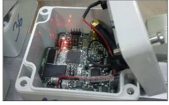
Figure 1. SMAMID Functional Unit
Thus, we present a comprehensive review of some calibration
tests, partly documented in (D‟Urso, Crespi, Barbati, 2011) and of some additional sensitivity tests. The formers have been used to evaluate the most relevant parameters of systematic errors (bias, scale factor, thermal correction parameter) and accidental errors (noise) which are expressed in terms of standard deviation. The latter aim at estimating the variability of the offset and of the scale factor as function of different external environmental factors such as temperature and supply voltage. In the same operative conditions the offset values have been evaluated for all sensors as function of temperature; we have also checked if these variations are cyclic. In a further measurement session the scale factor has been evaluated between different sensors through static measurements. Finally, we have used the MEMS sensors as inclinometers for ISPRS Annals of the Photogrammetry, Remote Sensing and Spatial Information Sciences, Volume I-4, 2012
measuring and monitoring the inclination of elements which the sensors were fixed to, since time variation of the inclination is representative of the kinematics of the point at which the element and the sensor are bound. Purpose of the test was to ascertain which level of accuracy of inclination could be derived from accelerometer sensors by taking as reference values those imposed with a theodolite. In particular the values of inclination have been computed by using methods which combine the values of acceleration acquired on one or two axes of the sensor.
2. STATIC TEST
The proposed measurement system is made of a tern of tri-axial sensors; it allows for a high-resolution time monitoring of all state positioning whose output signal can be analyzed and modeled as function of characteristic parameters such as bias (ba), scale factor (sa), and thermal correction factor (cT). Such parameters are mainly due to the mechanical instability of the instruments or to physical disturbances of the environment. The tern of accelerometers is placed on a metal plate so as to permit a contemporary movement of the three sensors. Such a plate, fixed to a theodolite, can be regulated so that to establish a perfectly horizontal plane necessary for executing the static test of six faces illustrated in the sequel.
The parameters ba, sa,cT can be assumed as constant, with a value obtained by means a static measurement during a sufficiently long time interval. As a matter of fact, these parameters are not really constant since, otherwise they could be a-priori calibrated in laboratory by directly adjusting the observations. To determine the value of such parameters it is possible to invoke standard calibration procedures based on the measurement, for a conveniently long time, generally ten minutes, of a physical quantity such as the gravity acceleration. After estimating bias and scale factor it is possible to filter the signal.
In particular the state equation connecting the accelerometer measurement
z
a and the actual accelerationz
is temperature measurement, T0 the temperature lighting on sensor and ν the noise of observation.2.1 Calibration static test
The calibration test is a non-traditional low-cost procedure, aiming at determining the error-parameters.
The determination of the bias and of the scale-factor of the accelerometers has been carried out according to the standard IEEE 517 (Institute of Electrical and Electronical Engineers),
and known in the literature as “six positions static test” ( El-Sheimy et al., 2003, Titterton & Weston, 2004).
Clearly, for a successful realization of the test, the tern of sensors must lie on a horizontal plane: for this reason, a tripod with a geodetic base, put in station by means of a torus precision level, has been used. A put in station theodolite, connected to the perfectly horizontal metal plate, hosting the tern of accelerometers has been put on a tripod. During the test it was necessary to avoid disturbances to the measurements exerted by external agents, such as sudden accelerations or sensible temperature variations. This last parameter is the most difficult to control, since each sensor tends to get overheated
during its functioning.
The parameters estimated in this way represent the actual systematic error of the instrument and can be used to adjust the raw observations by simply reversing the error model.
During the test the inertial sensor has been put on a horizontal plane, and the axes of the reference system oriented up/down, alternatively, for all the six possible positions. To avoid errors during the adjustment data an exact rotation of 180 degrees, between two opposite faces of the sensor has been carried out so as to ensure that the vertical axis is exactly the same in the two cases. In this way one obtains an estimate of both bias and scale factor of the accelerometers by summing and subtracting the combinations of the inertial measurements.
Figure 2. Sensors in the ” z_ up” e “z_ down” configurations
Assuming that the noise of the observation has been removed from the model expressed in (1), as a consequence of a subsequent filtering, the equations of the vertical accelerometers in two possible configurations, are:
g accelerometer. The noise of the observations can be determined by means of the formulas:
g receive any current variation.
2.2 Results
The calibration procedure based on the “six positionsstatic test”
adopts a reference system coincident with the North, East and vertical axes.
The test has been carried out during two days by letting the sensor be fixed on every face for 15 minutes and spending, after every change of position, at least 5 further minutes to avoid ISPRS Annals of the Photogrammetry, Remote Sensing and Spatial Information Sciences, Volume I-4, 2012
placing the tern of accelerometers in open field in order to characterize the behaviour of the sensors as function of external temperature; during the test the value of 20°C has been recorded.
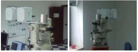
Figure 3. Equipment during calibration of the static test. Laboratory and open field tests
On the basis of the measured quantities, bias and scale factor of each sensor ranged about a value, averaged all over the measurement session, of 10-3g in each direction.
The components of the raw acceleration, adjusted with the average values of the bias and scale factor, are considerably
reduced and become closer to the theoretical value “1g”. Vice -versa the raw data of the accelerometers are sensibly reduced for the adjustment of the scale factor.
Once the systematic errors have been computed, the values of the static, raw acceleration are represented in Figure 4 for a session of measurement of 10 seconds.
984
Data correction for systematic error FU SMAMID n.03
Orignal data up
Correct data up
Figure 4. Laboratory static test - Observations adjusted from systematic errors – session acquisition of 10 seconds
The analysis of precision carried out for the parameters of the three sensors, equipped with the relative graphics, shows a substantial stability of the systematic parameters during the measurement. Apart from particular operative cases, e.g. those related to significant temperature variations, it is reasonable to assume that the theoretical assumption (Sansò, 2006) according to which systematic parameters can be considered constant during sessions of measurement of 1-2 hours holds true. In conclusion, it is necessary to repeat the calibration procedures, at regular time intervals, as function of frequency and of the use of the sensors; in this way a realistic estimate of the error parameters is obtained.
By modifying the values of the frequency, from 40Hz to 160Hz and 640Hz, and the values of the scale from, ±2g to ±6g, we heve obtained a lot of time-information; specifically, a particularly jammed signal and an increase of the instrumental error. The best configuration has been obtained with the values 40Hz and ±2g, with a s.q.m. equal to 10-4g; vice-versa we have
obtained a s.q.m. equal to 10-3g by varying the frequency of acquisition.
2.3 Sensibility and sensitivity analysis
Further tests have been carried out to take into account the different operative conditions concerning laboratory and open field (outside). For instance Figure 5 shows the comparison of the average values of bias (offset) and scale factor for laboratory and open field tests.
Figure 5. Average values of bias and scale-factor for laboratory and open field calibration tests
Clearly, the error of greater interest is the scale factor since it cannot be a-priori corrected with knowing in advance its variation as function of the external parameters. MEMS sensors of the SMAMID FUs have a digital output expressed in bits and each output is converted to quantities measured in terms of the gravity acceleration g by means of a conversion factor (sensitivity) acting on the Less Significant bit (LSb). Such a conversion factor is typical of any of the three axes of each FU and ranges in a definite interval (974-1074 with prevalence of 1024 LSb/g) reported in the data sheet provided by manufacturer.
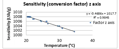
The results of the tests have shown that such a value does not change as function of the sampling frequency and of the measurement range. Moreover it turns out to be insensitive both to run-to-run variations and to measurement sessions carried out at different hours and constant temperatures. Conversely, tests carried out inside and outside the laboratory exhibit a variation with temperature. For this reason a temperature–controlled test has been carried out by measuring the value of interest with a temperature sensor placed inside the SMAMID FU and repeating the measurement by exposing the unit to sunlight or shading it. It is clear from Figure 6 that the scale factor significantly reduces as temperature increases by following approximately a linear law. As a matter of fact variation ranges about 0.045% °C by taking also into account the error of the temperature sensor placed inside the FU.
y = -0.4686x + 1017.7
Figure 6. Sensitivity for z axis with temperature variation.
We may thus conclude that temperature plays a significant role, especially if the FUs need to operate in the open field, even if it represents the unique parameter affecting the value of the scale factor over time. Actually, it is significant to point out that the scale factor attains its initial value whenever the FU is shaded and temperature keeps constant.
The additional important parameter is bias, i.e. the deviation of the signal output from the null value which should be attained when no acceleration is applied. Whenever constant, bias can be eliminated by averaging the measurements; however, it has to be taken into account that the offset values are different between the axes of each FU since they depend upon the assembly. To this end some further measurements have been carried out and it has been concluded that the offset values:
a) do belong to the interval reported in the data sheet provided by the sensor manufacturer;
b) are different for each axis but do not change as function of additional setting parameters or run-to-run effects;
c) are constant over time only for short periods and their variation as function of environmental factors is not negligible.
A further important quantity which cannot be individuated by the static test is the sensor resolution; in this specific case it can be assumed equal to precision. The variation of the results obtained in the static test as function of the sampling frequency and of the full scale depend upon the instrumental resolution which, in turn, depend upon such parameters in the sense that they tend to get worse as the sampling frequency and the full scale increase. Moreover, the resolution is different between the transversal directions and the vertical one. The sum up the setting–up operations have allowed us to conclude that the adopted instrumentation behaves coherently with the parameters reported in the data sheet provided by the manufacturer; however, some additional parameters exhibit a degree of indeterminacy so high as to require characterization tests, specific for each axis of each FU, which also take into account temperature changes.
Thus, a future objective of the research will be concerned with the implementation of an adjustment algorithm accounting for the variations of the temperature as well as for the systematic and casual errors.
3. VARIOMETRY TESTS OF MEMS SENSORS USED AS INCLINOMETERS
One of the main objectives of the proposed SMAMID–based measurement system is to use it as inclinometers. Specifically, by fixing the system to a rigid object, the sensors allow one to measure and monitor the inclination of elements which they are fixed to, since time variation of the inclination is representative of the kinematics of the point at which the element and the sensor are bound. This application is significant in the geomatic low-cost monitoring techniques, particularly in determining slope movements during landslides, at least in the superficial part of the slope. Purpose of the test was to ascertain which level of accuracy of inclination could be derived from accelerometer sensors by taking as reference values those imposed with a theodolite. In particular the value of inclination have been computed using methods which combine the values of acceleration on one or two axes of the sensor.
3.1 Experimental set-up
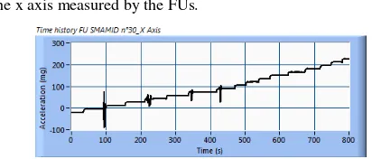
The test apparatus consists of three SMAMID FUs fixed to a Wild T2 theodolite. Starting from an initial condition of 300 gon for the zenith angle, variations of the angle have been imposed, with a step of 1 gon in the range 300-284 gon, and the relevant accelerations measured by three tri-axial MEMS sensors. In particular, angles can be measured by means of a tri-axial accelerometer by evaluating the variation of the gravity acceleration along the three axes. For instance Figure 7 shows as function of time the tendency of the acceleration values along
the x axis measured by the FUs.
Figure 7. Time history for FU SMAMID n°30 x axis during zenith angle variation from 300 to 284 gon.
Points when sudden increments of the accelerations do occur correspond to the instants of time in which the inclination of the collimation axis of the theodolite, hence of the x-axis of the
FUs, changes. The “steps” in the signal output do indicate a transition between different system states; moreover one can notice time intervals, lasting a few seconds, in which the inclination of the collimation axis has been kept constant so that the acceleration has not changed. Accordingly, the acceleration content which keeps constant in a given time interval can be extracted very simply by taking the average of all the samplings at that time; in this way random variations, noise and disturbances can be eliminated from the signal. To this end the acceleration measure, corrected of the bias, can be obtained in variometric terms by employing initial values as reference. Inclination can be computed by different approaches depending on the fact that the accelerations measured on different axes are combined or not.
3.2Uni-axial method
The first step in each measurement session is a pre-elaboration of the datum; it amounts to expressing accelerations in the desired measurement units, to correcting undesired effects (such as impulsive effects which modify the collimations axis and jam the acquisition of the static acceleration) and to extracting, see e.g. Figure 7, the records pertaining to the time intervals in which the collimation axis does not change or is not affected by any kind of disturbance. The subsequent step is concerned with the evaluation of the static acceleration of an axis around which a rotation does happen.
It is worth noting that sensors of the SMAMID FU are able to record both phenomena of static nature, such as acceleration constant over time, and dynamic phenomena of oscillatory type within the frequency range made available by the sampling frequency, e.g. 20 Hz in our case.
By selecting time interval of length T in which the theodolite is fixed, one can compute an average value of the static acceleration in the x direction during the time T, say it
x
A.Such a value accounts not only of the component x of the gravity acceleration, Axg, but also of the bias Axoff which needs to be evaluated and eliminated from the measurements:
xg xoff
x
A
A
A
(5)Assuming an initial measurement as reference value and that the offset value does not change significantly among the measurements carried out at different values of angular inclination (i.e. at different time instants) one can obtain the variation of inclination by difference. For instance, suppose one wants to evaluate the inclination by means of the acceleration signal in the x direction corresponding to a zenith angle of 299 gon; to this end let us consider the plots of the time intervals in Figure 8 in which the collimation angle of the theodolite is set ISPRS Annals of the Photogrammetry, Remote Sensing and Spatial Information Sciences, Volume I-4, 2012
to 300 and 299 gon.
Figure 8. Time history x axis extraction at 300 gon (left) and at 299 gon (right)
Starting from these two series the average values of accelerations Ax(300) and Ax(299), can be computed. By
considering the reference frame of the test and that accelerations are expressed in terms of the gravity acceleration g, so that the total modulus of the accelerations keeps constantly equal to 1g, one can simply write: possible to assume that the sensor is horizontal when the test is carried out with a zenith angle of 300 gon, it is sufficient to correct the acceleration attained at the inclination of 299 gon of the value Ax(300) obtained at the inclination of 300 gon, ( thus
assumed equal to the offset):
) 0.895°, corresponding approximately to 0.994 gon, value very close to the expected value of 1 gon. Thus, one can operate similarly for the other directions.
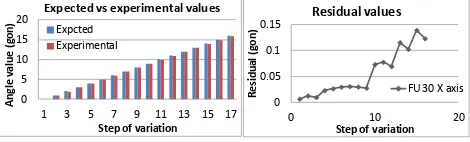
3.2.1 Results of the x-axis approach: The previously illustrated approach allows one to compute all the inclinations. Results are summarized in Figure 9 showing the measured angular values, i.e. those derived from the acceleration, and the expected ones, i.e. those imposed to the theodolite.
0
Figure 9. Tilt values one axis x mode Expected versus experimental values (left) residual (rigth)
One infers from Figure 9 that the differences are really negligible with a slight underestimate in the values derived from the accelerations. In particular, one notices in the second plot of Figure 9 that the absolute deviation between the real value, provided by theodolite, and the measured one does increase with inclination. The average value of the deviation is approximately equal to 0.05 gon and it has been obtained as average of the deviation attained for the three FUs at different inclinations. By considering 1mg resolution value for the
acceleration one would have a minimum value of angular resolution equal to 0.07 gon. Thus the average deviations are in accordance with this error.
3.2.2 Results of the z-axis approach: One notices from Figure 10 the typical step-wise tendency, clearly visible on the z component, only after five angular variations: the acceleration is almost constant with the exception of the instants at which the collimation angle changes and the FUs are affected by dynamical effects.
Figure 10.Time history for FU SMAMID n°30 z axis during zenith variation from 300 to 284 gon
As before, the formula to adopt is:
)
Figure 11. Tilt values one axis z mode. Expected vs experimental values (left) - residual (right)
Differently from the x and the y axis, for which the resolution error is equal to 1mg, the first value of inclination which can be derived from the z axis , i.e. 0.997g,corresponds to a variation significant differences with respect to the expected values. The deviation has a definite tendency to diminish as the inclination increases.
3.3 Biaxial method
Comparing the deviation values which are obtained by the two methods one notices that the error achieved with the x-axis acceleration tends to increase as the inclination increases; on the contrary for the z-axis the deviation tends to slightly reduce as the variation increases. To try to compensate such effects one can employs the tangent function which employs both measurement axes at the same time. In this case the formula to adopt in order to evaluate the inclination is:
( )/ ( )
increases with inclination. By considering all the angular ISPRS Annals of the Photogrammetry, Remote Sensing and Spatial Information Sciences, Volume I-4, 2012variations imposed during the experimental tests, the deviation between the expected and actual angular values, these last one being evaluated by means of the accelerations measured along the x-axis, is approximatively equal to 0.05 gon; this value has to be intended as the average between the three FUs.
0 5 10 15 20
1 3 5 7 9 11 13 15 17
A
n
g
le
v
a
lu
e
(
g
o
n
)
Step of variation Expected vs experimental values
Expcted Experimental
0 0.1 0.2 0.3
0 10 20
R
e
si
d
u
a
l
(g
o
n
)
Step of variation Residual values
FU 30 biaaxil
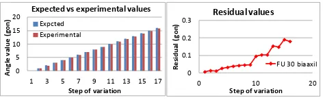
Figure 12. Tilt values for biaxial mode. Experimental values (left) - residual (right)
By employing the biaxial method above for the same experimental data, one achieves an absolute deviation of 0.08 gon. In any case by assuming, as a first approximation, an instrumental error of 0.07 gon, it is possible to conclude that, as an average, both the uni-axial method along the x axis and the bi-axial method do provide inclinations comparable with those imposed to the theodolite. As a matter of fact the uni-axial method along the x axis is certainly the most effective one for small inclinations; however, it is reasonable to state that approaching inclinations of 45°, preference should be credited to the biaxial method. By virtue of these results one can conclude that the bi-axial method can exhibit the considerable advantage of being applicable over a broader range of inclinations.
4. CONCLUSIONS
Experimental tests carried out at the Cassino University have proved the correct functioning of the SMAMID measurement system, i.e. a system composed of an independent Functional Unit (FU), each one equipped with a tri-axial accelerometer, controlled in a wireless mode by a personal computer. Any tests have been carried out both in laboratory and in open field using a master and three FU sensors, what allowed us to obtain estimates of the most relevant errors (bias or offset, scale factor, sensitivity). The values of acceleration measured in laboratory are lower than those measured in open field, reversing the trend of the temperatures. Generally, a decrease of the temperature (in open field) generates an increase of the average values relative to bias and to scale factor. Vice-versa, an accidental error as the noise presents a swinging trend and increases with temperature. Moreover, it has been checked that suitable processes of data treatment allowed us to use the acceleration recorded by the FUs for extracting information on the inclination. A variometric test of inclination within the x-z plane has been carried out by recording the accelerations of the three FUs fixed to a theodolite for which a 1 gon increment of zenith angle has been assigned in the interval 300-284 gon.
Experimental results have been processed by two different approaches: the first one has employed the acceleration measured by each FU along a single axis; the second one has tried to combine the accelerations pertaining to two axes. By taking into account all the angular variations considered during the experimental tests it is possible to state preliminarily that, as an average, both the uni-axial and the biaxial method do provide values of inclinations comparable to those imposed to the theodolite as reference value. Moreover, the biaxial method is useful for angular variations spanning the whole range of measurements for the inclination. Conversely, by choosing the
axis less influenced by the gravity component, and hence affected by a reduced error, the uni-axial method turns out to be more adequate for small angle deviations.
Such method could be usefully applied to a network of SMAMID accelerometers, acting as inclinometers, in order to exploit a multisensor and distributed approach as well as the advantages of the wireless connection and the battery supply: thus, it could represent an interesting measurement system in geomatics for monitoring slow phenomena such as landslides. Some aspects related to the error and to the precision of such elaboration methods still require further study in order to better understand their limits and to optimize their applications. In this respect further measurements sessions will be carried out in order to test the proposed system over a broader range of inclinations and to employ further traditional instruments for measuring angles such as inclinometers and total stations. Thus, in order to fully exploit the potentialities of such kind of sensors, it is necessary to adopt several calibration procedures aiming at an exhaustive modelling the behaviour of the different types of systematic errors.
5. REFERENCES
D‟Urso, M.G., Crespi, M., Barbati, N., 2011. Una prova di sensibilità di sensori accelerometrici triassiali, Atti 15a Conferenza Nazionale ASITA, Reggia di Colorno.
El-Sheimy, N., Nassar, S., Noureldin, A., 2004. Wavelet De-Noising for IMU Alignment, IEEE A&E System Magazine, pp.32-39.
Jekeli, C., 2001. Inertial Navigation Systems with Geodetic Applications. de Gruyter, Berlino - New York.
Khichar, R., Shivanandan, S., 2002. "Wireless sensor networks and their applications in geomatics: case study on developments in developing countries". Applied Geomatics, 2: pp.43-48 http://www.springerlink.com.
Sansò, F., 2006. „Navigazione geodetica e rilevamento
cinematico‟, Polipress, Milano.
Titterton, D.H., Weston, J.L., 2004. Strapdown inertial navigation technology. IEEE American Institute of Aeronautics
Tuck, K., 2007. Tilt Sensing Using Linear Accelerometers
journal Sensors Free scale SemiconductorAN3461, Rev.1 n.05.
Acknowledgements
We warmfully thank prof. Mattia Crespi, University of Rome La Sapienza, for his kind support and helpful suggestions, and eng. Giovanni Mannara, vice-president of STRAGO S.p.A, for providing us with the experimental equipment.