f37 book intarch pres pt3

Jan. 2011

Computer Architecture, The

Arithmetic/Logic Unit

Slide 1

Part III

Jan. 2011

Computer Architecture, The

Arithmetic/Logic Unit

Slide 2

About This Presentation

This presentation is intended to support the use of the textbook

ComputerArchitecture:FromMicroprocessorstoSupercomputers, Oxford University Press, 2005, ISBN 0-19-515455-X. It is updated regularly by the author as part of his teaching of the

upper-division course ECE 154, Introduction to Computer Architecture, at the University of California, Santa Barbara. Instructors can use these slides freely in classroom teaching and for other

educational purposes. Any other use is strictly prohibited. © BehroozParhami

Edition Released Revised Revised Revised Revised

First July 2003 July 2004 July 2005 Mar. 2006 Jan. 2007

Jan. 2011

Computer Architecture, The

Arithmetic/Logic Unit

Slide 3

III The Arithmetic/Logic Unit

Topics in This Part

Chapter 9 Number Representation

Chapter 10 Adders and Simple ALUs

Chapter 11 Multipliers and Dividers

Chapter 12 Floating-Point Arithmetic

Overview of computer arithmetic and ALU design:

Jan. 2011

Computer Architecture, The

Arithmetic/Logic Unit

Slide 4

Preview of Arithmetic Unit in the Data Path

Fig. 13.3 Key elements of the single-cycle MicroMIPS data path.

/

ALU _cache Data

Instr cache Next addr Reg file op jta fn inst imm

rs (rs)

(rt) Data addr Data in 0 1 ALUSrc

ALUFunc DataWrite DataRead SE RegInSrc rt rd RegDst RegWrite 32 / 16 Register input Data out Func ALUOvfl Ovfl 31 0 1 2 Next PC Incr PC (PC) Br&Jump ALU out PC 0 1 2

Instruction fetch Reg access / decode ALU operation Data access

Jan. 2011

Computer Architecture, The

Arithmetic/Logic Unit

Slide 5

Computer Arithmetic as a Topic of Study

Brief overview article –

Encyclopedia of Info Systems, Academic Press, 2002,

Vol. 3, pp. 317-333

Our textbook’s treatment of the topic falls between the extremes (4 chaps.)

Graduate course ECE 252B – Text:

Jan. 2011

Computer Architecture, The

Arithmetic/Logic Unit

Slide 6

9 Number Representation

Arguably the most important topic in computer arithmetic:

• Affects system compatibility and ease of arithmetic

• Two’s complement, flp, and unconventional methods

Topics in This Chapter

9.1 Positional Number Systems 9.2 Digit Sets and Encodings 9.3 Number-Radix Conversion 9.4 Signed Integers

Jan. 2011

Computer Architecture, The

Arithmetic/Logic Unit

Slide 7

9.1 Positional Number Systems

Representations of natural numbers {0, 1, 2, 3, …}

||||| ||||| ||||| ||||| ||||| || sticks or unary code

27 radix-10 or decimal code

11011 radix-2 or binary code

XXVII Roman numerals

Fixed-radix positional representation with

k

digits

Value of a number: x = (x_k–1x_k–2 . . . x₁x₀)_r =



x_i r i For example:

27 = (11011)_two = (124) + (1_23) + (0_22) + (1_21) + (120₎

Number of digits for [0, P]: k = log_r (P + 1) = log_r P + 1

k–1

Jan. 2011

Computer Architecture, The

Arithmetic/Logic Unit

Slide 8

Unsigned Binary Integers

Figure 9.1 Schematic representation of 4-bit code for integers in [0, 15].

0000 0001 1111 0010 1110 0011 1101 0100 1100 1000 0101 1011 0110 1010 0111 1001 0 1 2 3 4 5 6 7 15 11 14 13 12 8 9 10

Inside: Natural number Outside: 4-bit encoding

0 1 2 3 15 4 5 6 7 8 9

Turn x notches counterclockwise

to add x

Turn y notches clockwise to subtract y

11 14 13 12

Jan. 2011

Computer Architecture, The

Arithmetic/Logic Unit

Slide 9

Representation Range and Overflow

Figure 9.2 Overflow regions in finite number representation systems. For unsigned representations covered in this section, max – = 0.

max

Finite set of representable numbers

Overflow region

max

Overflow region

Numbers larger than max

Numbers smaller than max

  

  

Example 9.2, Part d

Discuss if overflow will occur when computing 317 – 316 in a number system with k = 8 digits in radix r = 10.

Solution

Jan. 2011

Computer Architecture, The

Arithmetic/Logic Unit

Slide 10

9.2 Digit Sets and Encodings

Conventional and unconventional digit sets



Decimal digits in [0, 9]; 4-bit BCD, 8-bit ASCII



Hexadecimal, or hex for short: digits 0-9 & a-f



Conventional ternary digit set in [0, 2]

Conventional digit set for radix

r

is [0,

r

– 1]

Symmetric ternary digit set in [–1, 1]



Conventional binary digit set in [0, 1]

Redundant digit set [0, 2], encoded in 2 bits

( 0 2 1 1 0 )

Jan. 2011

Computer Architecture, The

Arithmetic/Logic Unit

Slide 11

Carry-Save Numbers

Radix-2 numbers using the digits 0, 1, and 2

Example: (1 0 2 1)_two = (123) + (0_22) + (2_21) + (1_20) = 13 Possible encodings

(a) Binary (b) Unary

0 00 0 00

1 01 1 01 (First alternate)

2 10 1 10 (Second alternate)

11 (Unused) 2 11

1 0 2 1 1 0 2 1

Jan. 2011

Computer Architecture, The

Arithmetic/Logic Unit

Slide 12

Figure 9.3 Adding a binary number or another

carry-save number to a carry-save number.

The Notion of Carry-Save Addition

Two carry-save

inputs Carry-save

input

Binary input

Carry-save output

This bit being 1 represents

overflow (ignore it)

0 0

0

a. Carry-save addition. b. Adding two carry-save numbers.

Carry-save addition

Carry-save addition

Jan. 2011

Computer Architecture, The

Arithmetic/Logic Unit

Slide 13

9.3 Number Radix Conversion



Perform arithmetic in the new radix

R

Suitable for conversion from radix r to radix 10

Horner’s rule:

(x_k–1x_k–2 . . . x₁x₀)_r = (…((0 + x_k–1)r + x_k–2)r + . . . + x₁)r + x₀

(1 0 1 1 0 1 0 1)_two = 0 + 1  1  2 + 0  2  2 + 1  5  2 + 1 

11  2 + 0  22  2 + 1  45  2 + 0  90  2 + 1  181



Perform arithmetic in the old radix

r

Suitable for conversion from radix 10 to radix R

Divide the number by R, use the remainder as the LSD and the quotient to repeat the process

19 / 3  rem 1, quo 6 / 3  rem 0, quo 2 / 3  rem 2, quo 0

Thus, 19 = (2 0 1)_three

Jan. 2011

Computer Architecture, The

Arithmetic/Logic Unit

Slide 14

Justifications for Radix Conversion Rules

Figure 9.4 Justifying one step of the conversion of x to radix 2.

x 0

x mod 2 Binary representation of x/2

Justifying Horner’s rule.

1 2

1 2 0 1 2 1 0

(

x x

_{k k}

x

)

_r

x r

_k k

x r

_k k

x r x

 

L











L





0

(

1

(

2

( )))

x

r x

r x

r

Jan. 2011

Computer Architecture, The

Arithmetic/Logic Unit

Slide 15

9.4 Signed Integers



We dealt with representing the natural numbers



Signed or directed whole numbers = integers

{ . . . , 3, 2, 1, 0, 1, 2, 3, . . . }



Signed-magnitude representation

+27 in 8-bit signed-magnitude binary code 0 0011011 –27 in 8-bit signed-magnitude binary code 1 0011011 –27 in 2-digit decimal code with BCD digits 1 0010 0111



Biased representation

Represent the interval of numbers [N, P] by the unsigned

Jan. 2011

Computer Architecture, The

Arithmetic/Logic Unit

Slide 16

Two’s-Complement Representation

Figure 9.5 Schematic representation of 4-bit 2’s-complement code for integers in [–8, +7].

0000 0001 1111 0010 1110 0011 1101 0100 1100 1000 0101 1011 0110 1010 0111 1001 +0 +1 +2 +3 +4 +5 +6 +7 �1 �5 �2 �3 �4 �8 �7 �6

+

_

0

1 2 3 �1 4 5 6 7 �8 �7

Turn x notches counterclockwise

to add x

Turn 16 �y notches counterclockwise to

add �y (subtract y) �5

�2

�3

�4

�6

Jan. 2011

Computer Architecture, The

Arithmetic/Logic Unit

Slide 17

Conversion from 2’s-Complement to Decimal

Example 9.7

Convert x = (1 0 1 1 0 1 0 1)_2’s-compl to decimal.

Solution

Given that x is negative, one could change its sign and evaluate –x. Shortcut: Use Horner’s rule, but take the MSB as negative

–1  2 + 0  –2  2 + 1  –3  2 + 1  –5  2 + 0  –10  2 +

1  –19  2 + 0  –38  2 + 1  –75

Example 9.8

Sign Change for a 2’s-Complement Number

Given y = (1 0 1 1 0 1 0 1)_2’s-compl, find the representation of –y.

Solution

Jan. 2011

Computer Architecture, The

Arithmetic/Logic Unit

Slide 18

Two’s-Complement Addition and Subtraction

Figure 9.6 Binary adder used as 2’s-complement adder/subtractor.

Add



Sub

x



y

y

x

k

/

k

/

k

/

y

or

y



Adder

c

_out

c

_in

k

Jan. 2011

Computer Architecture, The

Arithmetic/Logic Unit

Slide 19

9.5 Fixed-Point Numbers

Positional representation:

k

whole and

l

fractional digits

Value of a number: x = (x_k–1x_k–2. . .x₁x₀.x_–1x_–2 . . . x_–l )_r =



x_i r i For example:

2.375 = (10.011)_two = (121) + (0_20) + (0_21) + (1_22) + (1_23) Numbers in the range [0, rk _{– ulp] representable, where ulp = r}–l

Fixed-point arithmetic same as integer arithmetic (radix point implied, not explicit)

Jan. 2011

Computer Architecture, The

Arithmetic/Logic Unit

Slide 20

Fixed-Point 2’s-Complement Numbers

Figure 9.7 Schematic representation of 4-bit 2’s-complement encoding for (1 + 3)-bit fixed-point numbers in the range [–1, +7/8].

0.000

0.001 1.111

0.010 1.110

0.011 1.101

0.100 1.100

1.000

0.101 1.011

0.110 1.010

0.111 1.001

+0

+.125

+.25

+.375

+.5

+.625

+.75

+.875

�.125

�.625

�.25

�.375

�.5

�1

�.875

�.75

Jan. 2011

Computer Architecture, The

Arithmetic/Logic Unit

Slide 21

Radix Conversion for Fixed-Point Numbers



Perform arithmetic in the new radix

R

Evaluate a polynomial in r–1_{: (.011)}

two = 0  2–1 + 1  2–2 + 1  2–3

Simpler: View the fractional part as integer, convert, divide by rl

(.011)_two = (?)_ten

Multiply by 8 to make the number an integer: (011)_two = (3)_ten

Thus, (.011)_two = (3 / 8)_ten = (.375)_ten



Perform arithmetic in the old radix

r

Multiply the given fraction by R, use the whole part as the MSD and the fractional part to repeat the process

(.72)_ten = (?)_two

0.72  2 = 1.44, so the answer begins with 0.1

0.44  2 = 0.88, so the answer begins with 0.10

Convert the whole and fractional parts separately.

Jan. 2011

Computer Architecture, The

Arithmetic/Logic Unit

Slide 22

9.6 Floating-Point Numbers



Fixed-point representation must sacrifice precision

for small values to represent large values

x

= (0000 0000

.

0000 1001)

_two

Small number

y

= (1001 0000

.

0000 0000)

_two

Large number



Neither

y

2

nor

y

/

x

is representable in the format above



Floating-point representation is like scientific notation:



20 000 000 =



2

 107 +

0.000 000 007 = +7

_ 10–9

Useful for applications where very large and very small

numbers are needed simultaneously

Also, 7E9

Significand Exponent base Exponent

Jan. 2011

Computer Architecture, The

Arithmetic/Logic Unit

Slide 23

ANSI/IEEE Standard Floating-Point Format (IEEE 754)

Figure 9.8 The two ANSI/IEEE standard floating-point formats.

Short (32-bit) format

Long (64-bit) format

Sign Exponent Significand

8 bits, bias = 127,

�126 to 127

11 bits,

bias = 1023,

�1022 to 1023 52 bits for fractional part _{(plus hidden 1 in integer part)} 23 bits for fractional part

(plus hidden 1 in integer part)

Short exponent range is –127 to 128 but the two extreme values are reserved for special operands

(similarly for the long format)

Jan. 2011

Computer Architecture, The

Arithmetic/Logic Unit

Slide 24

Short and Long IEEE 754 Formats: Features

Table 9.1 Some features of ANSI/IEEE standard floating-point formats

Feature Single/Short Double/Long

Word width in bits 32 64

Significand in bits 23 + 1 hidden 52 + 1 hidden Significand range [1, 2 – 2–23_{] [1, 2 – 2}–52_]

Exponent bits 8 11

Exponent bias 127 1023

Zero (±0) e + bias = 0, f = 0 e + bias = 0, f = 0 Denormal e + bias = 0, f ≠ 0

represents ±0.f  2–126 erepresents ±0. + bias = 0, f ≠ 0f _ 2–1022

Infinity (∞) e + bias = 255, f = 0 e + bias = 2047, f = 0

Not-a-number (NaN) e + bias = 255, f ≠ 0 e + bias = 2047, f ≠ 0 Ordinary number e + bias  [1, 254]

e  [–126, 127]

represents 1.f  2e

e + bias  [1, 2046]

e  [–1022, 1023]

represents 1.f  2e

Jan. 2011

Computer Architecture, The

Arithmetic/Logic Unit

Slide 25

10 Adders and Simple ALUs

Addition is the most important arith operation in computers:

• Even the simplest computers must have an adder

• An adder, plus a little extra logic, forms a simple ALU

Topics in This Chapter

10.1 Simple Adders

10.2 Carry Propagation Networks 10.3 Counting and Incrementation 10.4 Design of Fast Adders

Jan. 2011

Computer Architecture, The

Arithmetic/Logic Unit

Slide 26

10.1 Simple Adders

Figures 10.1/10.2 Binary half-adder (HA) and full-adder (FA).

x y c s

0 0 0 0 0 1 0 1 1 0 0 1 1 1 1 0

Inputs Outputs

HA

x y

c

s

x y c c s

0 0 0 0 0 0 0 1 0 1 0 1 0 0 1 0 1 1 1 0 1 0 0 0 1 1 0 1 1 0 1 1 0 1 0 1 1 1 1 1

Inputs Outputs

c _out c _in

out

in _{x y}

s

FA

Digit-set interpretation: {0, 1} + {0, 1}

= {0, 2} + {0, 1}

Jan. 2011

Computer Architecture, The

Arithmetic/Logic Unit

Slide 27

Full-Adder Implementations

Figure10.3 Full adder implemented with two half-adders, by means of two 4-input multiplexers, and as two-level gate network.

(a) FA built of two HAs

(c) Two-level AND-OR FA (b) CMOS mux-based FA

1

0

3

2

HA

HA

1

0

3

2

0

1

x y

x y

x y

s

s s

c _out

c _out c _out

c _in

Jan. 2011

Computer Architecture, The

Arithmetic/Logic Unit

Slide 28

Ripple-Carry Adder: Slow But Simple

Figure 10.4 Ripple-carry binary adder with 32-bit inputs and output. x

s y

c c

x

s y

c

x

s y

c

c _out c in

0 0

0

c ₀

1 1

1

1 2

31

31

31 31

FA FA FA

32

. . .

Jan. 2011

Computer Architecture, The

Arithmetic/Logic Unit

Slide 29

Carry Chains and Auxiliary Signals

Bit positions

15 14 13 12 11 10 9 8 7 6 5 4 3 2 1 0 1 0 1 1 0 1 1 0 0 1 1 0 1 1 1 0

c_out 0 1 0 1 1 0 0 1 1 1 0 0 0 0 1 1 c_in

\__________/\__________________/ \________/\____/ 4 6 3 2

Carry chains and their lengths

Jan. 2011

Computer Architecture, The

Arithmetic/Logic Unit

Slide 30

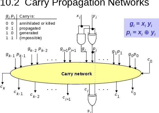
[image:30.720.118.633.46.412.2]

10.2 Carry Propagation Networks

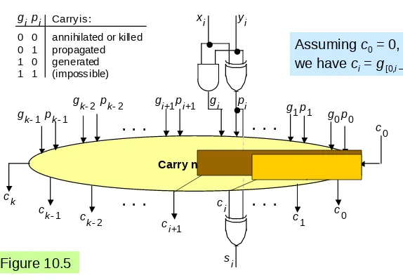
Figure 10.5 The main part of an adder is the carry network. The rest is just a set of gates to produce the g and p signals and the sum bits.

Carry network

. . .

. . .

x _i y _i

g p

s i i

i c _i

c _i+1 c _k1

c _k

c _k2 c ₁

c ₀ g p _{1 1}

g p _{0 0} g _k2 p _k2 g p _{i+1 i+1}

g _k1 p _k1

c ₀

. . .

. . .

0 0 0 1 1 0 1 1

annihilated or killed propagated

generated (impossible) Carry is: g _i p _i

Jan. 2011

Computer Architecture, The

Arithmetic/Logic Unit

Slide 31

Ripple-Carry Adder Revisited

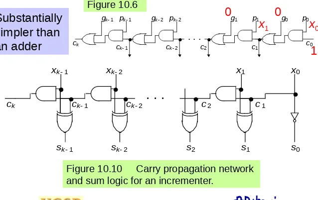
Figure 10.6 The carry propagation network of a ripple-carry adder.

. . .

c _k1

c _{k c}

k2 c 1

g ₁ p ₁ g ₀ p ₀ g k2 p _k2

g k1 p _k1

c ₀ c ₂

The carry recurrence:

c

_i+1

= g

_i



p

_i

c

_i

Latency of k-bit adder is roughly 2k gate delays:

1 gate delay for production of p and g signals, plus 2(k – 1) gate delays for carry propagation, plus

Jan. 2011

Computer Architecture, The

Arithmetic/Logic Unit

Slide 32

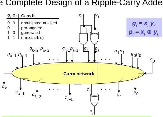
[image:32.720.113.637.48.424.2]

The Complete Design of a Ripple-Carry Adder

Figure 10.6 (ripple-carry network) superimposed on Figure 10.5 (general structure of an adder).

Carry network

. . .

. . .

x _i y _i

g p

s i i

i c _i

c _i+1 c _k1

c _k

c _k2 c ₁

c ₀ g p _{1 1}

g p _{0 0} g _k2 p _k2 g p _{i+1 i+1}

g _k1 p _k1

c ₀

. . .

. . .

0 0 0 1 1 0 1 1

annihilated or killed propagated

generated (impossible) Carry is: g _i p _i

Jan. 2011

Computer Architecture, The

Arithmetic/Logic Unit

Slide 33

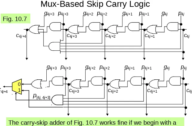
First Carry Speed-Up Method: Carry Skip

Figures 10.7/10.8 A 4-bit section of a ripple-carry network with skip paths and the driving analogy.

c

g 4j+1 p 4j+1 g 4j p 4j

g 4j+2 p 4j+2

g 4j+3 p 4j+3

c 4j

4j+4 c 4j+3 c 4j+2 c 4j+1

One-way street

Jan. 2011

Computer Architecture, The

Arithmetic/Logic Unit

Slide 34

Mux-Based Skip Carry Logic

The carry-skip adder of Fig. 10.7 works fine if we begin with a clean slate, where all signals are 0s; otherwise, it will run into problems, which do not exist in this mux-based implementation

c

g _4j+1 p _4j+1 g _4j p _4j g _4j+2 p _4j+2

g _4j+3 p _4j+3

c 4j

4j+4 c 4j+3 c 4j+2 c 4j+1

0 1

p_{[4j, 4j+3]} c_4j+4

c

g 4j+1 p 4j+1 g 4j p 4j

g 4j+2 p 4j+2

g 4j+3 p 4j+3

c 4j

[image:34.720.52.673.28.436.2]

4j+4 c 4j+3 c 4j+2 c 4j+1

Jan. 2011

Computer Architecture, The

Arithmetic/Logic Unit

Slide 35

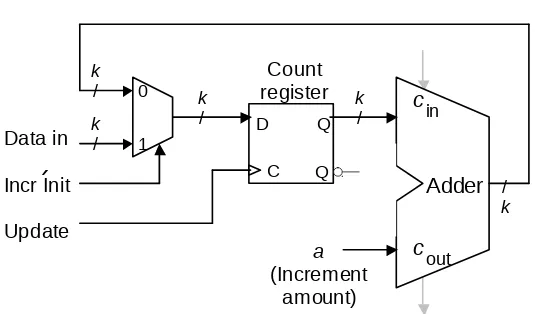
[image:35.720.91.626.103.417.2]

10.3 Counting and Incrementation

Figure 10.9 Schematic diagram of an initializable synchronous counter.

D Q

C

_

Q D

c

_out

c

_in

Adder

Update

/

k k

/

a

(Increment amount) Count

register _k

/ 1

0

Data in

k

/

k

/

Jan. 2011

Computer Architecture, The

Arithmetic/Logic Unit

Slide 36

Circuit for Incrementation by 1

[image:36.720.48.686.98.500.2]

Substantially

simpler than

an adder

Figure 10.10 Carry propagation network and sum logic for an incrementer.

1 0

k2 k1

. . .

c k1

c k c k2 c 1

x x

x x

c 2

1 0

k2

k1 s s s

s s 2

. . .

c k1

c k _c

k2 c 1

g 1 p 1 g 0 p 0

g k2 p k2

g k1 p k1

c 0

c 2

0

0

x

₀

x

₁

Figure 10.6

Jan. 2011

Computer Architecture, The

Arithmetic/Logic Unit

Slide 37



Carries can be computed directly without propagation



For example, by unrolling the equation for

c

₃

, we get:

c₃ = g₂  p₂ c₂ = g₂  p₂ g₁  p₂ p₁ g₀  p₂ p₁ p₀ c₀



We define “generate” and “propagate” signals for a block

extending from bit position

a

to bit position

b

as follows:

g_[a,b] = g_b  p_b g_b–1  p_b p_b–1g_b–2  . . .  p_b p_b–1…p_a+1 g_a

p_[a,b] = p_b p_b–1. . . p_a+1 p_a



Combining

g

and

p

signals for adjacent blocks:

g_[h,j] = g_[i+1,j]  p_[i+1,j] g_[h,i]

p_[h,j] = p_[i+1,j] p_[h,i]

10.4 Design of Fast Adders

h i

i+1

j

Jan. 2011

Computer Architecture, The

Arithmetic/Logic Unit

Slide 38

[image:38.720.73.647.74.473.2]

Carries as Generate Signals for Blocks [

0,

i

]

Figure 10.5

Carry network

. . .

. . .

x _i y _i

g p

s

i i

i

c _i c _i+1

c _k1 c _k

c _k2 c ₁

c ₀ g p _{1 1}

g p _{0 0} g _k2 p _k2 g p _{i+1 i+1}

g _k1 p _k1

c ₀

. . .

. . .

0 0 0 1 1 0 1 1

annihilated or killed propagated

generated (impossible) Carry is:

g _i p _i

Jan. 2011

Computer Architecture, The

Arithmetic/Logic Unit

Slide 39

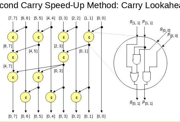
[image:39.720.75.647.39.428.2]

Second Carry Speed-Up Method: Carry Lookahead

Figure 10.11 Brent-Kung lookahead carry network for an 8-digit adder, along with details of one of the carry operator blocks.

¢ ¢ ¢ ¢

¢ ¢

¢ ¢

¢ ¢ ¢

[7, 7 ] [6, 6 ] [5, 5 ] [4, 4 ] [3, 3] [2, 2 ] [1, 1 ] [0, 0]

[0, 7 ] [0, 6 ] [0, 5 ] [0, 4 ] [0, 3] [0, 2 ] [0, 1 ] [0, 0] [2, 3]

[4, 5 ] [6, 7 ]

[4, 7 ]

[0, 3]

[0, 1 ]

g _{[0, 0]}

g _{[0, 1]} g _{[1, 1]}

p _{[0, 0]}

Jan. 2011

Computer Architecture, The

Arithmetic/Logic Unit

Slide 40

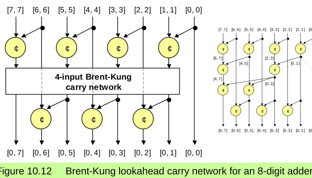
[image:40.720.45.674.87.445.2]

Recursive Structure of Brent-Kung Carry Network

Figure 10.12 Brent-Kung lookahead carry network for an 8-digit adder, with only its top and bottom rows of carry-operators shown.

¢ ¢ ¢ ¢

¢ ¢ ¢

[7, 7] [6, 6] [5, 5] [4, 4] [3, 3] [2, 2] [1, 1] [0, 0]

[0, 7] [0, 6] [0, 5] [0, 4] [0, 3] [0, 2] [0, 1] [0, 0]

4-input Brent-Kung carry network

¢ ¢ ¢ ¢

¢ ¢

¢ ¢

¢ ¢ ¢

[7, 7] [6, 6 ] [5, 5] [4, 4] [3, 3] [2, 2 ] [1, 1] [0, 0 ]

[0, 7] [0, 6 ] [0, 5] [0, 4] [0, 3] [0, 2 ] [0, 1] [0, 0 ] [2, 3 ]

[4, 5] [6, 7 ]

[4, 7 ]

[0, 3 ]

[0, 1 ]

g _{[0, 0]}

g _{[0, 1]} g _{[1, 1]}

p _{[0, 0]}

Jan. 2011

Computer Architecture, The

Arithmetic/Logic Unit

Slide 41

An Alternate Design: Kogge-Stone Network

Kogge-Stone lookahead carry network for an 8-digit adder.

¢ ¢ ¢ ¢

¢ ¢ ¢ ¢

¢ ¢

¢ ¢ ¢ ¢

¢

¢ ¢

c₁ = g_[0,0]

c₂ = g_[0,1]

c₃ = g_[0,2]

c₈ = g_[0,7] c₄ = g_[0,3]

c₅ = g_[0,4]

c₆ = g_[0,5]

Jan. 2011

Computer Architecture, The

Arithmetic/Logic Unit

Slide 42

¢ ¢ ¢ ¢

¢ ¢

¢ ¢

¢ ¢ ¢

[7, 7 ] [6, 6 ] [5, 5 ] [4, 4 ] [3, 3 ] [2, 2 ] [1, 1 ] [0, 0 ]

[0, 7 ] [0, 6 ] [0, 5 ] [0, 4 ] [0, 3 ] [0, 2 ] [0, 1 ] [0, 0 ] [2, 3 ]

[4, 5 ] [6, 7]

[4, 7]

[0, 3 ]

[0, 1 ]

g _{[0, 0]}

g _{[0, 1]} g _{[1, 1]}

p _{[0, 0]}

p _{[0, 1]} p _{[1, 1]}

Brent-Kung vs. Kogge-Stone Carry Network

11 carry operators 4 levels

Jan. 2011

Computer Architecture, The

Arithmetic/Logic Unit

Slide 43

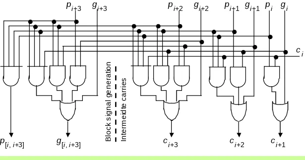
[image:43.720.49.664.105.428.2]

Carry-Lookahead Logic with 4-Bit Block

Figure 10.13 Blocks needed in the design of carry-lookahead adders with four-way grouping of bits.

B

lo

ck

s

ig

n

a

l g

e

n

e

ra

tio

n

p _{[i, i+3]}

c _i

In

te

rm

e

id

te

c

a

rr

ie

s

c _i+1 c _i+2

c _i+3 g _{[i, i+3]}

Jan. 2011

Computer Architecture, The

Arithmetic/Logic Unit

Slide 44

Third Carry Speed-Up Method: Carry Select

Figure 10.14 Carry-select addition principle.

c _out c _in

Adder

Version 1 of sum bits

1 0

x

[a, b]

c _out c _in

Adder

Version 0 of sum bits

y

[a, b]

s

[a, b]

c

a

0 1

Allows doubling of adder width with a single-mux additional delay

The lower

a positions, (0 to a – 1)

Jan. 2011

Computer Architecture, The

Arithmetic/Logic Unit

Slide 45

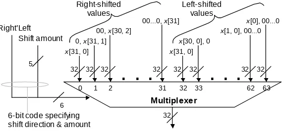
10.5 Logic and Shift Operations

[image:45.720.72.645.152.417.2]

Conceptually, shifts can be implemented by multiplexing

Figure 10.15 Multiplexer-based logical shifting unit.

Multiplexer

0 1 2 31 32 33 62 63

5

6

Right’Left

Shift amount _{0, x[31, 1]}

x[31, 0]

00, x[30, 2]

00...0, x[31]

x[31, 0]

x[30, 0], 0

x[1, 0], 00...0

x[0], 00...0

. . .

. . .

32

32 32 32 32 32 32 32 32

6-bit code specifying shift direction & amount

Right-shifted values

Jan. 2011

Computer Architecture, The

Arithmetic/Logic Unit

Slide 46

[image:46.720.52.656.140.437.2]

Arithmetic Shifts

Figure 10.16 The two arithmetic shift instructions of MiniMIPS.

Purpose: Multiplication and division by powers of 2

sra $t0,$s1,2 # $t0  _{($s1) right-shifted by 2}

srav $t0,$s1,$s0 # $t0  _{($s1) right-shifted by ($s0)}

1 1

1 1

0 0 0

fn

0 0 0 0 0 0 0 0 0 0 0 1 0 0

0 0 0 0 0 0 1 0 0 0 1 1 0

31 25 20 15 0

ALU

instruction Unused register Source

op rs rt

R

rd sh

10 5

Destination

register amount Shift sra = 3

1

0 0 0 0 0 0 0 0 0 0 0 0 0 0 0

0 0 1 0 0 0 0 1 0 0 0 1 1 0

31 25 20 15 0

ALU instruction

Amount register

Source register

op rs rt

R

rd sh

10 5 fn

Destination register

Jan. 2011

Computer Architecture, The

Arithmetic/Logic Unit

Slide 47

Practical Shifting in Multiple Stages

Figure 10.17 Multistage shifting in a barrel shifter.

2

0, x[31, 1]

x[31, 0]

x[30, 0], 0

32

0 1 2 3

32 32 32 32

0 0 No shift 0 1 Logical left 1 0 Logical right

1 1 Arith right x[31], x[31, 1]

Multiplexer

2

0 1 2 3

(0 or 4)-bit shift

2

0 1 2 3

(0 or 2)-bit shift

2

0 1 2 3

(0 or 1)-bit shift

(a) Single-bit shifter (b) Shifting by up to 7 bits

y[31, 0]

Jan. 2011

Computer Architecture, The

Arithmetic/Logic Unit

Slide 48

Figure 10.18 A 4



8 block of a black-and-white

image represented as a 32-bit word.

Bit Manipulation via Shifts and Logical Operations

AND with mask to isolate a field: 0000 0000 0000 0000 1111 1100 0000 0000

Right-shift by 10 positions to move field to the right end of word

The result word ranges from 0 to 63, depending on the field pattern

32-pixel (4  8) block of

black-and-white image:

1010 0000 0101 1000 0000 0110 0001 0111

Representation as 32-bit word:

Hex equivalent: _0xa0a80617

Row 0 Row 1 Row 2 Row 3

Jan. 2011

Computer Architecture, The

Arithmetic/Logic Unit

Slide 49

10.6 Multifunction ALUs

General structure of a simple arithmetic/logic unit.

Logic unit Arith

unit ₀

1

Operand 1

Operand 2

Result

Logic fn (AND, OR, . . .) Arith fn (add, sub, . . .)

Jan. 2011

Computer Architecture, The

Arithmetic/Logic Unit

Slide 50

An ALU for

MiniMIPS

Figure 10.19 A multifunction ALU with 8 control signals (2 for

function class, 1 arithmetic, 3 shift, 2 logic) specifying the operation.

AddSub

x y

y x

Adder

c ₃₂ c ₀

k / Shifter Logic unit s Logic function Amount 5 2 Constant amount Variable amount 5 5

ConstVar

0 1 0 1 2 3 Function class 2 Shift function

5 LSBs _{Shifted y} 32

32

32

2

c ₃₁

32-input NOR Ovfl Zero 32 32 MSB ALU y x s Shorthand symbol for ALU Ovfl Zero Func Control 0 or 1

AND 00 OR 01 XOR 10 NOR 11

00 Shift 01 Set less 10 Arithmetic 11 Logic 00 No shift

Jan. 2011

Computer Architecture, The

Arithmetic/Logic Unit

Slide 51

11 Multipliers and Dividers

Modern processors perform many multiplications & divisions:

• Encryption, image compression, graphic rendering

• Hardware vs programmed shift-add/sub algorithms

Topics in This Chapter

11.1 Shift-Add Multiplication 11.2 Hardware Multipliers

11.3 Programmed Multiplication 11.4 Shift-Subtract Division

Jan. 2011

Computer Architecture, The

Arithmetic/Logic Unit

Slide 52

11.1 Shift-Add Multiplication

Figure 11.1 Multiplication of 4-bit numbers in dot notation.

Multiplicand

Partial products bit-matrix

x y

z

y x 2 0 0

y x 2 1 1

y x 2 2 2

y x 2 3 3

Multiplier

Product

z

(j+1)

= (

z

(j)

+

y

j

x

2

k

) 2

–1

with

z

(0)

= 0 and

z

(k)

=

z

|––– add –––|

Jan. 2011

Computer Architecture, The

Arithmetic/Logic Unit

Slide 53

Binary and Decimal Multiplication

Figure 11.2 Step-by-step multiplication examples for 4-digit unsigned numbers.

Position 7 6 5 4 3 2 1 0 Position 7 6 5 4 3 2 1 0

========================= =========================

x24 _{1 0 1 0 x10}4 _{3 5 2 8}

y 0 0 1 1 y 4 0 6 7

========================= =========================

z(0) _{0 0 0 0 z}(0) _{0 0 0 0}

+y₀x24 _{1 0 1 0 +y}

0x104 2 4 6 9 6

–––––––––––––––––––––––––– ––––––––––––––––––––––––––

2z(1) _{0 1 0 1 0 10z}(1) _{2 4 6 9 6}

z(1) _{0 1 0 1 0 z}(1) _{0 2 4 6 9 6}

+y₁x24 _{1 0 1 0 +y}

1x104 2 1 1 6 8

–––––––––––––––––––––––––– ––––––––––––––––––––––––––

2z(2) _{0 1 1 1 1 0 10z}(2) _{2 3 6 3 7 6}

z(2) _{0 1 1 1 1 0 z}(2) _{2 3 6 3 7 6}

+y₂x24 _{0 0 0 0 +y}

2x104 0 0 0 0 0

–––––––––––––––––––––––––– ––––––––––––––––––––––––––

2z(3) _{0 0 1 1 1 1 0 10z}(3) _{0 2 3 6 3 7 6}

z(3) _{0 0 1 1 1 1 0 z}(3) _{0 2 3 6 3 7 6}

+y₃x24 _{0 0 0 0 +y}

3x104 1 4 1 1 2

–––––––––––––––––––––––––– ––––––––––––––––––––––––––

2z(4) _{0 0 0 1 1 1 1 0 10z}(4) _{1 4 3 4 8 3 7 6}

z(4) _{0 0 0 1 1 1 1 0 z}(4) _{1 4 3 4 8 3 7 6}

========================= =========================

Jan. 2011

Computer Architecture, The

Arithmetic/Logic Unit

Slide 54

Two’s-Complement Multiplication

Figure 11.3 Step-by-step multiplication examples for 2’s-complement numbers.

Position 7 6 5 4 3 2 1 0 Position 7 6 5 4 3 2 1 0

========================= =========================

x24 _{1 0 1 0 x2}4 _{1 0 1 0}

y 0 0 1 1 y 1 0 1 1

========================= =========================

z(0) _{0 0 0 0 0 z}(0) _{0 0 0 0 0}

+y₀x24 _{1 1 0 1 0 +y}

0x24 1 1 0 1 0

–––––––––––––––––––––––––– ––––––––––––––––––––––––––

2z(1) _{1 1 0 1 0 2z}(1) _{1 1 0 1 0}

z(1) _{1 1 1 0 1 0 z}(1) _{1 1 1 0 1 0}

+y₁x24 _{1 1 0 1 0 +y}

1x24 1 1 0 1 0

–––––––––––––––––––––––––– ––––––––––––––––––––––––––

2z(2) _{1 0 1 1 1 0 2z}(2) _{1 0 1 1 1 0}

z(2) _{1 1 0 1 1 1 0 z}(2) _{1 1 0 1 1 1 0}

+y₂x24 _{0 0 0 0 0 +y}

2x24 0 0 0 0 0

–––––––––––––––––––––––––– ––––––––––––––––––––––––––

2z(3) _{1 1 0 1 1 1 0 2z}(3) _{1 1 0 1 1 1 0}

z(3) _{1 1 1 0 1 1 1 0 z}(3) _{1 1 1 0 1 1 1 0}

+(–y₃x24_{) 0 0 0 0 0 +(–y}

3x24) 0 0 1 1 0

–––––––––––––––––––––––––– ––––––––––––––––––––––––––

2z(4) _{1 1 1 0 1 1 1 0 2z}(4) _{0 0 0 1 1 1 1 0}

z(4) _{1 1 1 0 1 1 1 0 z}(4) _{0 0 0 1 1 1 1 0}

========================= =========================

Jan. 2011

Computer Architecture, The

Arithmetic/Logic Unit

Slide 55

11.2 Hardware Multipliers

Multiplier y

Mux

Adder

out c

0 1

Doublewidth partial product z

Multiplicand x

Shift Shift

(j)

j

y

Add’Sub

Enable

Select

[image:55.720.135.572.49.458.2]

in c

Figure 11.4 Hardware multiplier based on the shift-add algorithm.

Jan. 2011

Computer Architecture, The

Arithmetic/Logic Unit

Slide 56

The Shift Part of Shift-Add

Figure11.5 Shifting incorporated in the connections to

the partial product register rather than as a separate phase.

out

c

To adder

y

_j

From adder

Sum

Partial product

Multiplier

/ k � 1

/ k � 1

/ k

Jan. 2011

Computer Architecture, The

Arithmetic/Logic Unit

Slide 57

High-Radix Multipliers

Radix-4 multiplication in dot notation.

Multiplicand x

y

z

Multiplier

Product

0, x, 2x, or 3x

z

(j+1)

= (

z

(j)

+

y

j

x

2

k

) 4

–1

with

z

(0)

= 0 and

z

(k/2)

=

z

|––– add –––|

Jan. 2011

Computer Architecture, The

Arithmetic/Logic Unit

Slide 58

[image:58.720.86.630.77.451.2]

Tree Multipliers

Figure 11.6 Schematic diagram for full/partial-tree multipliers.

Adder Large tree of

carry-save adders

. . .

All partial products

Product

Adder Small tree of

carry-save adders

. . .

Several partial products

Product

Log-depth

Log-depth

Jan. 2011

Computer Architecture, The

Arithmetic/Logic Unit

Slide 59

Array Multipliers

Figure 11.7 Array multiplier for 4-bit unsigned operands. 3 2 1 0 4 5 6 7 0 1 2 3

2 1 0

x x x

y y y z y 3

x 0 0 0 0 0 0 0 0 0 0 0 z z z z z z z HA FA FA MA MA MA MA MA MA MA MA MA MA MA MA MA MA MA MA FA 0 Our original dot-notation representing multiplication Straightened dots to depict array multiplier to the left

[image:59.720.93.684.43.473.2]

s

c

Jan. 2011

Computer Architecture, The

Arithmetic/Logic Unit

Slide 60

11.3 Programmed Multiplication

MiniMIPS instructions related to multiplication

mult $s0,$s1 # set Hi,Lo to ($s0)_{($s1); signed}

multu $s2,$s3 # set Hi,Lo to ($s2)_{($s3); unsigned}

mfhi $t0 # set $t0 to (Hi)

mflo $t1 # set $t1 to (Lo)

Finding the 32-bit product of 32-bit integers in MiniMIPS

Multiply; result will be obtained in _Hi,Lo For unsigned multiplication:

Hi should be all-0s and _Lo holds the 32-bit result For signed multiplication:

Jan. 2011

Computer Architecture, The

Arithmetic/Logic Unit

[image:61.720.84.615.121.424.2]

Slide 61

Figure 11.8 Register usage for programmed multiplication superimposed on the block diagram for a hardware multiplier.

Emulating a Hardware Multiplier in Software

$t2 (counter)

Part of the control in hardware Also, holds LSB of Hi during shift

Multiplier y

Mux

Adder

out c

0 1

Doublewidth partial product z

Multiplicand x

Shift Shift

(j)

j

y

Add’Sub

Enable

Select

in c

$a0 (multiplicand x)

$a1 (multiplier y)

$v1 (Lo part of z)

$v0 (Hi part of z)

$t0 (carry-out)

$t1 (bit j of y)

Jan. 2011

Computer Architecture, The

Arithmetic/Logic Unit

Slide 62

shamu: move $v0,$zero # initialize Hi to 0

move $vl,$zero # initialize Lo to 0

addi $t2,$zero,32 # init repetition counter to 32 mloop: move $t0,$zero # set c-out to 0 in case of no add

move $t1,$a1 # copy ($a1) into $t1

srl $a1,1 # halve the unsigned value in $a1 subu $t1,$t1,$a1 # subtract ($a1) from ($t1) twice to subu $t1,$t1,$a1 # obtain LSB of ($a1), or y[j], in $t1 beqz $t1,noadd # no addition needed if y[j] = 0

addu $v0,$v0,$a0 # add x to upper part of z

sltu $t0,$v0,$a0 # form carry-out of addition in $t0 noadd: move $t1,$v0 # copy ($v0) into $t1

srl $v0,1 # halve the unsigned value in $v0 subu $t1,$t1,$v0 # subtract ($v0) from ($t1) twice to subu $t1,$t1,$v0 # obtain LSB of Hi in $t1

sll $t0,$t0,31 # carry-out converted to 1 in MSB of $t0

addu $v0,$v0,$t0 # right-shifted $v0 corrected

srl $v1,1 # halve the unsigned value in $v1

sll $t1,$t1,31 # LSB of Hi converted to 1 in MSB of $t1

addu $v1,$v1,$t1 # right-shifted $v1 corrected

addi $t2,$t2,-1 # decrement repetition counter by 1

bne $t2,$zero,mloop # if counter > 0, repeat multiply loop jr $ra # return to the calling program

Multiplication When There Is No Multiply Instruction

Jan. 2011

Computer Architecture, The

Arithmetic/Logic Unit

Slide 63

11.4 Shift-Subtract Division

Figure11.9 Division of an 8-bit number by a 4-bit number in dot notation.

z

(j)

= 2

z

(j1)



y

kj

x

2

k

with

z

(0)

=

z

and

z

(k)

= 2

k

s

|

shift

|

|–– subtract ––|

2 1

2

y

2

x 2 2

1 0 3

0 Subtracted

bit-matrix Divisor

x

Dividend

z

s Remainder

Quotient

y

y x 3

y x 2

Jan. 2011

Computer Architecture, The

Arithmetic/Logic Unit

Slide 64

[image:64.720.59.653.40.516.2]

Integer and Fractional Unsigned Division

Figure 11.10 Division examples for binary integers and decimal fractions.

Position 7 6 5 4 3 2 1 0 Position –1 –2 –3 –4 –5 –6 –7 –8

========================= ==========================

z 0 1 1 1 0 1 0 1 z . 1 4 3 5 1 5 0 2

x24 _{1 0 1 0 x . 4 0 6 7}

========================= ==========================

z(0) _{0 1 1 1 0 1 0 1 z}(0) _{. 1 4 3 5 1 5 0 2}

2z(0) _{0 1 1 1 0 1 0 1 10z}(0) _{1 . 4 3 5 1 5 0 2}

–y₃x24 _{1 0 1 0 y}

3=1 –y–1x 1 . 2 2 0 1 y–1=3

–––––––––––––––––––––––––– –––––––––––––––––––––––––––

z(1) _{0 1 0 0 1 0 1 z}(1) _{. 2 1 5 0 5 0 2}

2z(1) _{0 1 0 0 1 0 1 10z}(1) _{2 . 1 5 0 5 0 2}

–y₂x24 _{0 0 0 0 y}

2=0 –y–2x 2 . 0 3 3 5 y–2=5

–––––––––––––––––––––––––– –––––––––––––––––––––––––––

z(2) _{1 0 0 1 0 1 z}(2) _{. 1 1 7 0 0 2}

2z(2) _{1 0 0 1 0 1 10z}(2) _{1 . 1 7 0 0 2}

–y₁x24 _{1 0 1 0 y}

1=1 –y–3x 0 . 8 1 3 4 y–3=2

–––––––––––––––––––––––––– –––––––––––––––––––––––––––

z(3) _{1 0 0 0 1 z}(3) _{. 3 5 6 6 2}

2z(3) _{1 0 0 0 1 10z}(3) _{3 . 5 6 6 2}

–y₀x24 _{1 0 1 0 y}

0=1 –y–4x 3 . 2 5 3 6 y–4=8

–––––––––––––––––––––––––– –––––––––––––––––––––––––––

z(4) _{0 1 1 1 z}(4) _{. 3 1 2 6}

s 0 1 1 1 s . 0 0 0 0 3 1 2 6

y 1 0 1 1 y . 3 5 2 8

========================= ==========================

Jan. 2011

Computer Architecture, The

Arithmetic/Logic Unit

Slide 65

[image:65.720.61.658.33.530.2]

Division with Same-Width Operands

Figure 11.11 Division examples for 4/4-digit binary integers and fractions.

Position 7 6 5 4 3 2 1 0 Position –1 –2 –3 –4 –5 –6 –7 –8

========================= ==========================

z 0 0 0 0 1 1 0 1 z . 0 1 0 1

x24 _{0 1 0 1 x . 1 1 0 1}

========================= ==========================

z(0) _{0 0 0 0 1 1 0 1 z}(0) _{. 0 1 0 1}

2z(0) _{0 0 0 1 1 0 1 2z}(0) _{0 . 1 0 1 0}

–y₃x24 _{0 0 0 0 y}

3=0 –y–1x 0 . 0 0 0 0 y–1=0

–––––––––––––––––––––––––– –––––––––––––––––––––––––––

z(1) _{0 0 0 1 1 0 1 z}(1) _{. 1 0 1 0}

2z(1) _{0 0 1 1 0 1 2z}(1) _{1 . 0 1 0 0}

–y₂x24 _{0 0 0 0 y}

2=0 –y–2x 0 . 1 1 0 1 y–2=1

–––––––––––––––––––––––––– –––––––––––––––––––––––––––

z(2) _{0 0 1 1 0 1 z}(2) _{. 0 1 1 1}

2z(2) _{0 1 1 0 1 2z}(2) _{0 . 1 1 1 0}

–y₁x24 _{0 1 0 1 y}

1=1 –y–3x 0 . 1 1 0 1 y–3=1

–––––––––––––––––––––––––– –––––––––––––––––––––––––––

z(3) _{0 0 0 1 1 z}(3) _{. 0 0 0 1}

2z(3) _{0 0 1 1 2z}(3) _{0 . 0 0 1 0}

–y₀x24 _{1 0 1 0 y}

0=0 –y–4x 0 . 0 0 0 0 y–4=0

–––––––––––––––––––––––––– –––––––––––––––––––––––––––

z(4) _{0 0 1 1 z}(4) _{. 0 0 1 0}

s 0 0 1 1 s . 0 0 0 0 0 0 1 0

y 0 0 1 0 y . 0 1 1 0

========================= ==========================

Jan. 2011

Computer Architecture, The

Arithmetic/Logic Unit

Slide 66

Signed Division

Method 1 (indirect): strip operand signs, divide, set result signs

Dividend Divisor Quotient Remainder z = 5 x = 3  y = 1 s = 2

z = 5 x = –3  y = –1 s = 2

z = –5 x = 3  y = –1 s = –2

z = –5 x = –3  y = 1 s = –2

Method 2 (direct 2’s complement): develop quotient with digits –1 and 1, chosen based on signs, convert to digits 0 and 1

Restoring division: perform trial subtraction, choose 0 for q digit if partial remainder negative

Jan. 2011

Computer Architecture, The

Arithmetic/Logic Unit

Slide 67

[image:67.720.127.598.48.439.2]

11.5 Hardware Dividers

Figure 11.12 Hardware divider based on the shift-subtract algorithm.

Load

Quotient y

Mux

Adder

0 1

Partial remainder z (initially z)

Divisor x

Shift Shift

(j)

k�j

y

1

Enable

Select

Quotient digit selector

1

out

c c_in

Trial difference (Always _subtract)

Jan. 2011

Computer Architecture, The

Arithmetic/Logic Unit

Slide 68

[image:68.720.83.606.109.366.2]

The Shift Part of Shift-Subtract

Figure 11.13 Shifting incorporated in the connections to the

partial remainder register rather than as a separate phase.

To adder

From adder

Partial remainder

Quotient

/ k

/ k / k

/ k

k�j

q

Jan. 2011

Computer Architecture, The

Arithmetic/Logic Unit

Slide 69

High-Radix Dividers

Radix-4 division in dot notation.

Divisor

x

Dividend

z

s Remainder

Quotient

y

0, x, 2x, or 3x

z

(j)

= 4

z

(j1)



(

y

k2j+1

y

k2j

)

two

x

2

k

with

z

(0)

=

z

and

z

(k/2)

= 2

k

s

|

shift

|

Jan. 2011

Computer Architecture, The

Arithmetic/Logic Unit

Slide 70

[image:70.720.46.673.66.444.2]

Array Dividers

Figure 11.14 Array divider for 8/4-bit unsigned integers.

2 1 0

x x x

1

y

2

y

3

y z 3

0 y 3 x 2 z 1 z 0 z 4 z 5 z 6 z 7 z MS MS MS MS MS MS MS MS MS MS MS MS MS MS MS MS Our original dot-notation for division Straightened dots to depict an array divider

2 1 0

s s s

Jan. 2011

Computer Architecture, The

Arithmetic/Logic Unit

Slide 71

11.6 Programmed Division

MiniMIPS instructions related to division

div $s0,$s1 # Lo = quotient, Hi = remainder

divu $s2,$s3 # unsigned version of division

mfhi $t0 # set $t0 to (Hi)

mflo $t1 # set $t1 to (Lo)

Compute z mod x, where z (singed) and x > 0 are integers

Divide; remainder will be obtained in _Hi if remainder is negative,

then add |x| to (_Hi) to obtain z mod x

else _Hi holds z mod x

Jan. 2011

Computer Architecture, The

Arithmetic/Logic Unit

[image:72.720.59.656.77.418.2]

Slide 72

Figure 11.15 Register usage for programmed division superimposed on the block diagram for a hardware divider.

Emulating a Hardware Divider in Software

Example 11.8 (MiniMIPS shift-add program for division)

Load

Quotient y

Mux

Adder

0 1

Partial remainder z (initially z)

Divisor x

Shift Shift

(j)

k�j

y

1

Enable

Select

Quotient digit selector 1

out

c c_in

Trial difference (Always _subtract)

$t2 (counter)

$a0 (divisor x)

$a1 (quotient y)

$v1 (Lo part of z)

$v0 (Hi part of z)

$t1 (bit kj of y)

Part of the control in hardware

Jan. 2011

Computer Architecture, The

Arithmetic/Logic Unit

Slide 73

shsdi: move $v0,$a2 # initialize Hi to ($a2)

move $vl,$a3 # initialize Lo to ($a3)

addi $t2,$zero,32 # initialize repetition counter to 32 dloop: slt $t0,$v0,$zero # copy MSB of Hi into $t0

sll $v0,$v0,1 # left-shift the Hi part of z slt $t1,$v1,$zero # copy MSB of Lo into $t1

or $v0,$v0,$t1 # move MSB of Lo into LSB of Hi sll $v1,$v1,1 # left-shift the Lo part of z

sge $t1,$v0,$a0 # quotient digit is 1 if (Hi)  _x,

or $t1,$t1,$t0 # or if MSB of Hi was 1 before shifting sll $a1,$a1,1 # shift y to make room for new digit or $a1,$a1,$t1 # copy y[k-j] into LSB of $a1

beq $t1,$zero,nosub # if y[k-j] = 0, do not subtract

subu $v0,$v0,$a0 # subtract divisor x from Hi part of z nosub: addi $t2,$t2,-1 # decrement repetition counter by 1

bne $t2,$zero,dloop # if counter > 0, repeat divide loop move $v1,$a1 # copy the quotient y into $v1

jr $ra # return to the calling program

Division When There Is No Divide Instruction

Jan. 2011

Computer Architecture, The

Arithmetic/Logic Unit

Slide 74

Load Quotient y Mux Adder

0 1

Partial remainder z (initially z)

Divisor x

Shift Shift

(j)

k�j

y 1 Enable Select Quotient digit selector 1 out

c c _in

Trial difference (Always _subtract)

Multiplier y

Mux

Adder out

c

0 1

Doublewidth partial product z

Multiplicand x

Shift Shift

(j)

j y Add’Sub Enable Select in c

Divider vs Multiplier: Hardware Similarities

2 1 0

x x x

1

y

2

y

3

y z 3

0 y 3 x 2 z 1 z 0 z 4 z 5 z 6 z 7 z MS MS MS MS MS MS MS MS MS MS MS MS MS MS MS MS Our original dot-notation for division Straightened dots to depict an array divider

2 1 0

s s s

[image:74.720.28.691.39.524.2]

3 s 0 0 0 0

Figure 11.12 Figure 11.4

3 2 1 0 4 5 6 7 0 1 2 3

2 1 0

x x x

y y y z y 3

x 0 0 0 0 0 0 0 0 0 0 0 z <