Electronic Journal of Qualitative Theory of Differential Equations
2009, No. 2, 1-15;http://www.math.u-szeged.hu/ejqtde/
THE GENERALIZED APPROXIMATION METHOD AND NONLINEAR HEAT TRANSFER EQUATIONS
RAHMAT ALI KHAN
Abstract. Generalized approximation technique for a solution of one-dimensional steady state heat transfer problem in a slab made of a material with temperature dependent thermal conductivity, is developed. The results obtained by the generalized approximation method (GAM) are compared with those studied via homotopy perturbation method (HPM). For this problem, the results ob-tained by the GAM are more accurate as compared to the HPM. Moreover, our (GAM) generate a sequence of solutions of linear problems that converges monotonically and rapidly to a solution of the original nonlinear problem. Each approximate solution is ob-tained as the solution of a linear problem. We present numerical simulations to illustrate and confirm the theoretical results.
1. Introduction
Fins are extended surfaces and are frequently used in various in-dustrial engineering applications to enhance the heat transfer between a solid surface and its convective, radiative environment. For surfaces with constant heat transfer coefficient and constant thermal conductiv-ity, the governing equation describing temperature distribution along the surfaces are linear and can be easily solved analytically. But most metallic materials have variable thermal properties, usually, depending
Key words and phrases. keywords; Heat transfer equation, Upper and lower so-lutions, Generalized approximation
Acknowledgement: Research is supported by HEC, Pakistan, Project 2-3(50)/PDFP/HEC/2008/1
The Author is thankful to the reviewer for his/her valuable comments and sugges-tions that lead to improve the original manuscript.
on temperature. The governing equations for the temperature distri-bution along the surfaces are nonlinear. In consequence, exact ana-lytic solutions of such nonlinear problems are not available in general and scientists use some approximation techniques such as perturba-tion method [1], [2], homotopy perturbaperturba-tion method [3], [4], [5] etc., to approximate the solutions of nonlinear equations as a series solu-tion. These methods have the drawback that the series solution may not always converges to the solution of the problem and hence produce inaccurate and meaningless results.
2. HEAT TRANSFER PROBLEM: HPM METHODS
When using perturbation methods, small parameter should be ex-erted into the equation to produce accurate results. But the exertion of a small parameter in to the equation means that the nonlinear effect is small and almost negligible. Hence, the perturbation method can be applied to a restrictive class of nonlinear problems and is not valid for general nonlinear problems.
It is claimed that the homoptopy perturbation method does not re-quire the existence of a small parameter and gives excellent results compared to the perturbation method for all values of the parameter, see for example [6, 7, 8]. In these papers, the authors discussed the solutions of temperature distributions in a slab with variable thermal conductivity and the two methods are compared in the field of heat transfer.
to homotopy perturbation. We use the computer programme, Mathe-matica.
Consider one-dimensional conduction in a slab of thickness L made of a material with temperature dependent thermal conductivity k =
k(T). The two faces are maintained at uniform temperatures T1 and T2 with T1 > T2. The governing equation describing the temperature
distribution
d dx(k
dT
dx) = 0, x∈[0, L], T(0) =T1, T(L) =T2.
(2.1)
see [8]. The thermal conductivity k is assumed to vary linearly with temperature, that is, k =k2[1 +η(T −T2)], where η is a constant and k2 is the thermal conductivity at temperature T2. After introducing
the dimensionless quantities
θ= T −T2
T1−T2, y = x
L, ǫ=η(T1−T2) =
k1−k2 k2 ,
where k1 is the thermal conductivity at temperature T1, the problem
(2.1) reduces to
−d
2θ
dy2 = ǫ(dθ
dy)
2
(1 +ǫθ) =f(θ, θ ′
), y ∈[0,1] = I,
θ(0) = 1, θ(1) = 0.
(2.2)
Three term expansion of the approximate solution of (2.2) by homotopy perturbation method is given by
(2.3) θ(y) = 1−y+ ǫ 2(y−y
2) +ǫ2(y2
− y
3
2 −
y
2), y∈I
see [8].
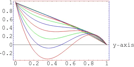
Results obtained for different values ofǫvia HPM (2.3) are presented in Table 1 and Fig. 1. Clearly, for small value for ǫ (ǫ ≤ 1), (2.3) is a good approximation to the solution. However, as ǫ increases, (2.3) deviates from the actual solution of the problem (2.2) and produce inaccurate results.
y 0.1 0.2 0.3 0.4 0.5 0.6 0.7 0.8 0.9
ǫ= 0.5 0.912375 0.824 0.734125 0.642 0.546875 0.448 0.344625 0.236 0.121375
ǫ= 0.8 0.91008 0.82304 0.73696 0.64992 0.56 0.46528 0.36384 0.25376 0.13312
ǫ= 1 0.9045 0.816 0.7315 0.648 0.5625 0.472 0.3735 0.264 0.1405
ǫ= 1.5 0.876375 0.776 0.692125 0.618 0.546875 0.472 0.386625 0.284 0.157375
ǫ= 2 0.828 0.704 0.616 0.552 0.5 0.448 0.384 0.296 0.172
ǫ= 2.5 0.759375 0.6 0.503125 0.45 0.421875 0.4 0.365625 0.3 0.184375
ǫ= 3 0.6705 0.464 0.3535 0.312 0.3125 0.328 0.3315 0.296 0.1945
ǫ= 3.5 0.561375 0.296 0.167125 0.138 0.171875 0.232 0.281625 0.284 0.202375
ǫ= 4 0.432 0.096 -0.056 -0.072 0. 0.112 0.216 0.264 0.208
[image:4.595.131.556.165.325.2]ǫ= 4.5 0.282375 -0.136 -0.315875 -0.318 -0.203125 -0.032 0.134625 0.236 0.211375
Table 1-Approximate solutions of (2.2) via HPM for different values ofǫ
0 0.2 0.4 0.6 0.8 1
-0.2 0 0.2 0.4 0.6 0.8 1
y-axis
Fig.1; Graphical results obtained via HPM for different values ofǫ.
3. HEAT TRANSFER PROBLEM: INTEGRAL
FORMULATION
We write (2.2) as an equivalent integral equation,
θ(y) = (1−y) +
Z 1
0
G(y, s)f(θ(s), θ′
(s))ds= (1−y) +
Z 1
0
G(y, s) ǫ(θ ′
)2
(1 +ǫθ)ds, (3.1)
where,
G(y, s) =
(
(1−s)y, 0≤y≤s≤1,
(1−y)s, 0≤s≤y≤1,
[image:4.595.195.419.371.483.2]is the Green’s function. Clearly,G(y, s)>0 on (0,1)×(0,1) and since
ǫ(θ′)2
(1+ǫθ) ≥0, hence, any solution θ of the BVP (2.2) is positive on I. We
recall the concept of lower and upper solutions.
Definition 3.1. A function α is called a lower solution of the BVP (2.2), if α∈C1(I) and satisfies
−α′′
(y)≤f(α(y), α′
(y)), y∈(0,1)
α(0)≤1, α(1)≤0.
An upper solution β ∈ C1(I) of the BVP (2.2) is defined similarly by reversing the inequalities.
For example, α= 1−y andβ = 2−y22 are lower and upper solutions of the BVP (2.2).
Definition 3.2. A continuous functionh: (0,∞)→(0,∞) is called a Nagumo function if
Z ∞
λ
sds
h(s) =∞,
for λ = max{|α(0)−β(1)|,|α(1)−β(0)|}. We say that f ∈C[R×R] satisfies a Nagumo condition relative toα, β if fory ∈[minα,maxβ] = [0,2], there exists a Nagumo functionh such that |f(y, y′
)| ≤h(|y′
|).
Clearly,
|f(θ, θ′
)|=| ǫ(
dθ dy)
2
(1 +ǫθ)| ≤ǫ|θ ′2
|=h(|θ′
|) for θ ∈[0,2]
and since R∞
λ sds h(s) =
R∞
λ sds
ǫs2 = ∞, where λ = 2 in this case. Hence f
satisfies a Nagomo condition. Existence of solution to the BVP (2.2) is guaranteed by the following theorem. The proof is on the same line as given in [9, 10] for more general problems.
Theorem 3.3. Assume that there exist lower and upper solutionsα, β ∈
C1(I) of the BVP (2.2) such that α ≤ β on I. Assume that f :
R×R→(0,∞)is continuous, satisfies a Nagumo condition and is non-increasing with respect to θ′. Then the BVP
positive solution θ such that α(y) ≤ θ(y) ≤ β(y), y ∈ I. Moreover, there exists a constantC depending onα, β andhsuch that|θ′
(y)| ≤C.
Using the relationRC
λ sds
h(s) ≥maxβ−minα = 2, we obtainC ≥2e 2ǫ.
In particular, we choose C = 2e2ǫ.
4. Heat Transfer Problem: Generalized Approximation
Method (GAM)
Observe that
fθθ(θ(s), θ′(s)) =
2ǫ3θ′2
(1 +ǫθ)3 ≥0, fθ′θ′(θ(s), θ
′
(s)) = 2ǫ
1 +ǫθ ≥0,
fθθ′(θ(s), θ′(s)) = − 2ǫ2θ′
(1 +ǫθ)2 and fθθfθ′θ′ =
4ǫ4θ′2
(1 +ǫθ)4 = (fθθ′) 2.
(4.1)
Hence, the quadratic form
vTH(f)v = (θ−z)2fθθ+ 2(θ−z)(θ′ −z′)fθθ′ + (θ′−z′)2fθ′θ′
=(θ−z)
s
ǫ3θ′2
(1 +ǫθ)3 −(θ
′
−z′ )
s
2ǫ
(1 +ǫθ)
2
≥0,
(4.2)
whereH(f) =
fθθ fθθ′
fθθ′ fθ′θ′
is the Hessian matrix andv =
θ−z θ′
−z′
.
Consequently,
f(θ, θ′
)≥f(z, z′
) +fθ(z, z
′
)(θ−z) +fθ′(z, z ′
)(θ′
−z′ ).
(4.3)
Define g :R4 →R by
g(θ, θ′ ; z, z′
) =f(z, z′
) +fθ(z, z′)(θ−z) +fθ′(z, z′)(θ′−z′), (4.4)
then g is continuous and satisfies the following relations
(4.5)
(
f(θ, θ′
)≥g(θ, θ′ ; z, z′
), f(θ, θ′
) =g(θ, θ′ ; θ, θ′
).
We note that for every θ, z ∈ [miny∈Iα, maxy∈Iβ] and z′ ∈ some
compact subset of R, g satisfies a Nagumo condition relative to α, β. Hence, there exists a constant C1 such that any solutionθ of the linear
BVP
−θ′′
(y) =g(θ, θ′ ; z, z′
), y ∈I, θ(0) = 1, θ(1) = 0,
with the property that α≤θ ≤β onI, must satisfies |θ′
|< C1 onI. To develop the iterative scheme, we choose w0 = α as an initial ap-proximation and consider the linear BVP
−θ′′
(y) =g(θ, θ′
; w0, w0′), y ∈I, θ(0) = 1, θ(1) = 0.
(4.6)
In view of (4.5) and the definition of lower and upper solutions, we obtain
g(w0, w′
0; w0, w0′) = f(w0, w0′)≥ −w
′′
0, g(β, β′
; w0, w′
0)≤f(β, β
′
)≤ −β′′
, on I,
which imply that w0 and β are lower and upper solutions of (4.6).
Hence, by Theorem 3.3, there exists a solution w1 of (4.6) such that w0 ≤ w1 ≤ β, |w1′| < C1 on I. Using (4.5) and the fact that w1 is a
solution of (4.6), we obtain
(4.7) −w′′
1(y) =g(w1, w1′; w0, w0′)≤f(w1, w1′)
which implies that w1 is a lower solution of (2.2). Similarly, we can show that w1 and β are lower and upper solutions of
−θ′′
(y) =g(θ, θ′
; w1, w1′), y ∈I, θ(0) = 1, θ(1) = 0.
(4.8)
Hence, there exists a solutionw2of (4.8) such thatw1 ≤w2 ≤β, |w2′|< C1 on I.
Continuing this process we obtain a monotone sequence {wn} of
solu-tions satisfying
α=w0≤ w1 ≤w2 ≤w3 ≤...≤wn−1 ≤wn ≤β, |wn|′ < C1 onI,
where wn is a solution of the linear problem
−θ′′
(y) =g(θ, θ′
; wn−1, w ′
n−1), y ∈I θ(0) = 1, θ(1) = 0
and is given by (4.9)
wn(y) = (1−y)+
Z 1
0
G(y, s)g(wn(s), wn′(s); wn−1(s), wn′−1(s))ds, y∈I.
The sequence is uniformly bounded and equicontinuous. The mono-tonicity and uniform boundedness of the sequence {wn} implies the
existence of a pointwise limit w on I. From the boundary conditions, we have
1 = wn(0)→w(0) and 0 =wn(1)→w(1).
Hencewsatisfies the boundary conditions. Moreover, by the dominated convergence theorem, for any y∈I,
Z 1
0
G(y, s)g(wn(s), wn′(s);wn−1(s), wn′−1(s))ds →
Z 1
0
G(y, s)f(w(s), w′
(s))ds.
Passing to the limit as n→ ∞, we obtain
w(y) = (1−y) +
Z 1
0
G(y, s)f(w(s), w′
(s))ds, y ∈I,
that is, wis a solution of (2.2).
Since α = 1 −y, β = 2 − y22 are lower and upper solutions of the problem (2.2). Hence, any solution θ of the problem satisfies 1−y ≤ θ ≤ 2− y22, y ∈ I. In other words, any solution of the problem is positive and is bounded by 2.
5. Convergence Analysis
Define en = w−wn on I. Then, en ∈ C1(I), en ≥0 on I and from
the boundary conditions, we have en(0) = 0 =en(1). In view of (4.5),
we obtain
−e′′
n(t) = f(w(t), w
′
(t))−g(wn(t), w
′
n(t);wn−1(t), wn′−1(t))≥0, t ∈I,
which implies that en is concave on I and there exists t1 ∈(0,1) such
that
(5.1) e′
n(t1) = 0, e′n(t)≥0 on [0, t1] and e′n(t)≤0 on [t1,1].
Using the definition of g and the non-increasing property of f(θ, θ′ ) with respect to θ, we have
−e′′
n(t) =f(w(t), w
′
(t))−g(wn(t), w
′
n(t);wn−1(t), w′n−1(t)), t∈I
=f(wn−1(t), wn′−1(t)) +fθ(wn−1(t), w′n−1(t))(w(t)−wn−1(t))
+fθ′(wn−1(t), w ′
n−1(t))(w
′
(t)−w′
n−1(t)) +
1 2v
TH(f)v
−g(wn(t), w′n(t);wn−1(t), w ′
n−1(t))
=fθ(wn−1(t), wn′−1(t))(w(t)−wn(t))+
fθ′(wn−1(t), w′n−1(t))(w ′
(t)−w′
n(t)) +
1 2v
TH(f)v
≤fθ′(wn−1(t), w ′
n−1(t))e
′
n(t) +
1 2v
TH(f)v,
where
vTH(f)v =(w−wn−1)
s
ǫ3ξ2 2
(1 +ǫξ1)3 −
(w′
−w′
n−1)
s
2ǫ
(1 +ǫξ1)
2
,
where wn−1 ≤ξ1 ≤wand ξ2 lies between w′n−1 and w ′
.
vTH(f)v ≤|en−1|C2ǫ√ǫ+|e′n−1|
√
2ǫ 2
≤ǫ(C2ǫ+√2)2ken−1k21 =dken−1k21,
whered=ǫ(C2ǫ+√2)2,C
2 = max{C, C1}andken−1k1 = max{ken−1k, ke′n−1k}
is the C1 norm. Hence,
−e′′
n(t)≤fθ′(wn−1(t), w′n−1(t))e
′
n(t) +
d
2ken−1k
2
1, t∈I,
which implies that
(5.2) (c1(t)e′
n(t))
′
≥ −dc12(t)ken−1k21, t ∈I,
where
c1(t) =eRfθ′(wn−1(t),wn′−1(t))dt = (1 +ǫw
n−1(t))2, t∈I.
Clearly 1≤c1(t)≤(1 +ǫ)2 onI. Integrating (5.2) from ttot1(t≤t1),
using e′
n(t1) = 0, we obtain
(5.3) e′
n(t)≤
dRt1
t c1(s)ds
2c1(t) k
en−1k21, t∈[0, t1]
and integrating (5.2) from t1 to t, we obtain
(5.4) e′
n(t)≥ −
dRtt
1c1(s)ds
2c1(t) k
en−1k21, t∈[t1,1].
From (5.3) and (5.4) together with (5.1), it follows that
(5.5) e′
n(t)≤
dRt1
t c1(s)ds
2c1(t) ken−1k
2 1 ≤
dR01c1(s)ds
2c1(t) ken−1k
2
1, t∈[0,1]
and (5.6)
e′
n(t)≥ −
dRt
t1c1(s)ds
2c1(t) ken−1k
2 1 ≥ −,
dR01c1(s)ds
2c1(t) ken−1k
2
1m, t∈[0,1].
Hence,
(5.7) ke′
nk ≤d1ken−1k21,
whered1 = max{
dR1 0 c1(s)ds
2c1(t) : t∈I}. Integrating (5.5) from 0 tot, using
the boundary conditione′
n(0) = 0 and taking the maximum overI, we
obtain
(5.8) kenk ≤d1ken−1k
2
1, t∈I.
From (5.7) and (5.8), it follows that
kenk1 ≤d1ken−1k21
which shows quadratic convergence.
6. NUMERICAL RESULTS FOR THE GAM
Starting with the initial approximationw0 = 1−y, results obtained
[image:10.595.122.482.165.538.2]of the choice of the parametersǫ involved, see Fig.5 .
y 0.1 0.2 0.3 0.4 0.5 0.6 0.7 0.8 0.9
w1 0.926897 0.850445 0.770062 0.685011 0.594355 0.496892 0.391076 0.274894 0.145703
w2 0.927888 0.852043 0.771941 0.68693 0.596178 0.498601 0.392748 0.276598 0.147208
w3 0.92791 0.852085 0.771998 0.686995 0.596245 0.498664 0.3928 0.276637 0.147228
[image:11.595.126.550.180.254.2]w4 0.927911 0.852086 0.772 0.686997 0.596247 0.498666 0.392802 0.276638 0.147229
Table 1; Results obtained via GAM for ǫ= 0.5
y 0.1 0.2 0.3 0.4 0.5 0.6 0.7 0.8 0.9
w1 0.923726 0.844367 0.761495 0.67454 0.582739 0.485077 0.38019 0.266234 0.140679
w2 0.924981 0.846597 0.764396 0.677808 0.586103 0.48832 0.38316 0.268796 0.142518
w3 0.925081 0.84679 0.764665 0.67813 0.586448 0.488658 0.38346 0.269028 0.14265
[image:11.595.124.553.330.401.2]w4 0.925091 0.846809 0.764692 0.678163 0.586484 0.488693 0.383491 0.269051 0.142664
Table 2; Results obtained via GAM for ǫ= 0.8
y 0.1 0.2 0.3 0.4 0.5 0.6 0.7 0.8 0.9
w1 0.921729 0.840541 0.756109 0.667965 0.575454 0.477674 0.373374 0.260812 0.137531
w2 0.923296 0.843436 0.760015 0.672516 0.580267 0.482379 0.377637 0.264317 0.139835
w3 0.923501 0.843836 0.760579 0.673195 0.581002 0.483104 0.378284 0.264818 0.140122
w4 0.923533 0.843898 0.760666 0.6733 0.581117 0.483218 0.378386 0.264896 0.140167
Table 3; Results obtained via GAM forǫ= 1
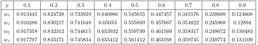
y 0.1 0.2 0.3 0.4 0.5 0.6 0.7 0.8 0.9
w1 0.913445 0.824728 0.733929 0.640986 0.545655 0.447457 0.345576 0.238689 0.124668
w1 0.916286 0.830217 0.741648 0.65033 0.555869 0.457667 0.354822 0.245968 0.12894
w1 0.917358 0.832312 0.744615 0.653932 0.559799 0.461569 0.358317 0.248672 0.130483
w1 0.917797 0.833171 0.745834 0.655412 0.561412 0.463168 0.359745 0.249774 0.131109
Table 4; Results obtained via GAM forǫ= 2
[image:11.595.128.552.458.532.2] [image:11.595.125.554.585.660.2]0 0.2 0.4 0.6 0.8 1 0
0.2 0.4 0.6 0.8 1
0 0.2 0.4 0.6 0.8 1
0 0.2 0.4 0.6 0.8 1
Fig.2. Results obtained by the GAM for ǫ = 0.5 (left graph) and
ǫ= 0.8 (right graph).
0 0.2 0.4 0.6 0.8 1
0 0.2 0.4 0.6 0.8 1
0 0.2 0.4 0.6 0.8 1
0 0.2 0.4 0.6 0.8 1
Fig.3. Results obtained by the GAM for ǫ = 1 (left graph) and ǫ = 2 (right graph).
0 0.2 0.4 0.6 0.8 1
0 0.2 0.4 0.6 0.8 1
0 0.2 0.4 0.6 0.8 1
0 0.2 0.4 0.6 0.8 1
Fig.4. Results obtained by the GAM for ǫ = 3 (left graph) and ǫ = 4 (right graph).
0 0.2 0.4 0.6 0.8 1 0
[image:13.595.196.426.113.261.2]0.2 0.4 0.6 0.8 1
Fig. 5; Graph of the results obtained by the GAM for ǫ= 0.5,0.8,1,2,3,4
7. Comparison with homotopy perturbation method
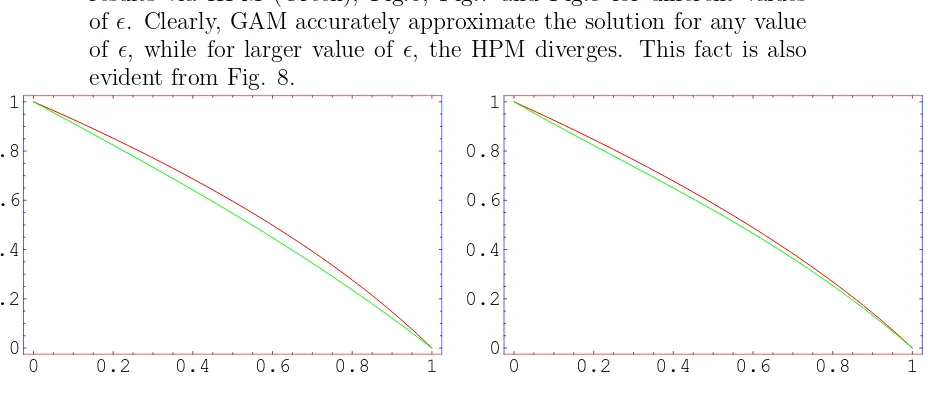
Finally, we compare results via GAM (Red) to the corresponding results via HPM (Green), Fig.6, Fig.7 and Fig.8 for different values of ǫ. Clearly, GAM accurately approximate the solution for any value of ǫ, while for larger value of ǫ, the HPM diverges. This fact is also evident from Fig. 8.
0 0.2 0.4 0.6 0.8 1
0 0.2 0.4 0.6 0.8 1
0 0.2 0.4 0.6 0.8 1
0 0.2 0.4 0.6 0.8 1
Fig.6. GAM and HPM for ǫ = 0.5 (left graph) and ǫ = 0.8 (right graph).
[image:13.595.82.546.467.673.2]0 0.2 0.4 0.6 0.8 1 0
0.2 0.4 0.6 0.8 1
0 0.2 0.4 0.6 0.8 1
0 0.2 0.4 0.6 0.8 1
Fig.7. GAM and HPM for ǫ= 1 (left graph) and ǫ = 2 (right graph).
0 0.2 0.4 0.6 0.8 1
0 0.1 0.2 0.3 0.4 0.5 0.6 0.7
0 0.2 0.4 0.6 0.8 1
0 0.2 0.4 0.6 0.8 1
Fig.8. GAM and HPM forǫ= 3 (left graph) and ǫ= 4 (right graph).
References
[1] M. Van Dyke, Perturbation Methods in Fluid Mechanics, Annotated Edition, Parabolic Press, Standford, CA, (1975).
[2] A. H. Nayfeh, Perturbation Methods, Wiley, New York, (1973).
[3] J. H. He, Homotopy perturbation technique,J. Comput. Methods Appl. Mech. Eng., 178(1999)(257), 3–4.
[4] J. H. He, A coupling method of a homotopy technique and a perturbation technique for non-linear problems,Int. J. Nonlinear Mech.,35(2000)(37).
[5] J. H. He, Homotopy perturbation technique,J. Comput. Methods Appl. Mech. Eng., 17(1999)(8), 257–262.
[6] D. D. Gunji, The application of He’s homotopy perturbation method to non-linear equations arising in heat transfer,Physics Letter A,355(2006), 337–341.
[7] D. D. Gunji and A. Rajabi, Assessment of homotopyperturbation and pertur-bation methods in heat radiation equations,Int. Commun. in Heat and Mass Transfer,33(2006), 391–400.
[8] A. Rajabi, D. D. Gunji and H. Taherian, Application of homotopy perturbation method in nonlinear heat conduction and convection equations,Physics Letter A,360(2007), 570–573.
[9] R. A. Khan and M. Rafique, Existence and multiplicity results for some three-point boundary value problems,Nonlinear Anal., 66(2007), 1686–1697.
[10] R. A. Khan, Generalized approximations and rapid convergence of solutions of
m-point boundary value problems, Appl. Math. Comput., 188 (2007), 1878– 1890.
(Received August 17, 2008)
Centre for Advanced Mathematics and Physics, National Univer-sity of Sciences and Technology(NUST), Campus of College of Elec-trical and Mechanical Engineering, Peshawar Road, Rawalpindi, Pak-istan,
E-mail address: rahmat [email protected]