SEMIDEFINITE GEOMETRY OF THE NUMERICAL RANGE∗
DIDIER HENRION†
Abstract. The numerical range of a matrix is studied geometrically via the cone of positive
semidefinite matrices (or semidefinite cone for short). In particular, it is shown that the feasible set of a two-dimensional linear matrix inequality (LMI), an affine section of the semidefinite cone, is always dual to the numerical range of a matrix, which is therefore an affine projection of the semidefinite cone. Both primal and dual sets can also be viewed as convex hulls of explicit algebraic plane curve components. Several numerical examples illustrate this interplay between algebra, geometry and semidefinite programming duality. Finally, these techniques are used to revisit a theorem in statistics on the independence of quadratic forms in a normally distributed vector.
Key words. Numerical range, Semidefinite programming, LMI, Algebraic plane curves.
AMS subject classifications.14H50, 14Q05, 47A12, 52A10, 90C22.
1. Notations and definitions. The numerical range of a matrix A∈Cn×n
is defined as
W(A) ={w∗
Aw∈C : w∈Cn, w∗
w= 1}.
(1.1)
It is a convex compact set of the complex plane which contains the spectrum ofA. It is also called the field of values; see [8, Chapter 1] and [12, Chapter 1] for elementary introductions. Matlab functions for visualizing numerical ranges are freely available from [3] and [11].
Let
A0=In, A1=
A+A∗
2 , A2=
A−A∗ 2i
(1.2)
with In denoting the identity matrix of size n and i denoting the imaginary unit.
Define
F(A) ={y∈P2+ : F(y) =y0A0+y1A1+y2A20}
(1.3)
∗Received by the editors March 8, 2009. Accepted for publication May 28, 2010. Handling Editor:
Shmuel Friedland.
†CNRS; LAAS; 7 avenue du colonel Roche, F-31077 Toulouse, France; Universit´e de Toulouse;
UPS, INSA, INP, ISAE; LAAS; F-31077 Toulouse, France ([email protected]); and Faculty of Electrical Engineering, Czech Technical University in Prague, Technick´a 4, CZ-16626 Prague, Czech Republic ([email protected]). Partially supported by project number 103/10/0628 of the Grant Agency of the Czech Republic.
with 0 meaning positive semidefinite (since A0, A1, A2 are Hermitian matrices,
F(y) has real eigenvalues for all y) and P2
+ denoting the oriented projective real plane (a model of the projective plane where the signs of homogeneous coordinates are significant, and which allows orientation, ordering and separation tests such as inequalities, see [18] for more details). Set F(A) is a linear section of the cone of positive semidefinite matrices (or semidefinite cone for short) [1, Chapter 4]. Inequal-ity F(y) 0 is called a linear matrix inequality (LMI). In the complex plane C, or
equivalently, in the affine real planeR2, setF(A) is a convex set including the origin, an affine section of the semidefinite cone.
Let
p(y) = det(y0A0+y1A1+y2A2) be a trivariate form of degreendefining the algebraic plane curve
P={y∈P2+ : p(y) = 0}.
(1.4)
Let
Q={x∈P2
+ : q(x) = 0} (1.5)
be the algebraic plane curve dual toP, in the sense that we associate to each point
y∈ P a pointx∈ Qof projective coordinatesx= (∂p(y)/∂y0, ∂p(y)/∂y1, ∂p(y)/∂y2). Geometrically, a point in Q corresponds to a tangent at the corresponding point in
Q, and conversely; see [19, Section V.8] and [7, Section 1.1] for elementary properties of dual curves.
Let V denote a vector space equipped with inner product h·,·i. If x and y are
vectors, then hx, yi = x∗
y. If X and Y are symmetric matrices, then hX, Yi = trace(X∗Y). Given a setK in V, its dual set consists of all linear maps from K to non-negative elements in R, namely,
K∗
={y∈V : hx, yi ≥0, x∈ K}.
Finally, the convex hull of a setK, denoted convK, is the set of all convex combinations of elements inK.
2. Semidefinite duality. After identifying CwithR2 orP2+, the first observa-tion is that numerical rangeW(A) is dual to LMI setF(A), and hence, it is an affine projection of the semidefinite cone.
Lemma 2.1. W(A) = F(A)∗
= {(hA0, Wi, hA1, Wi, hA2, Wi) ∈ P2+ : W ∈
Cn×n
Proof. The dual toF(A) is
F(A)∗ = {x : hx, yi=hF(y), Wi=P
khAk, Wiyk≥0, W 0}
= {x : xk=hAk, Wi, W 0},
an affine projection of the semidefinite cone. On the other hand, since w∗
Aw =
w∗
A1w+i w∗A2w, the numerical range can be expressed as
W(A) = {x= (w∗
A0w, w∗A1w, w∗A2w)}
= {x : xk=hAk, Wi, W 0, rankW = 1},
the same affine projection as above, acting now on a subset of the semidefinite cone, namely, the non-convex variety of rank-one positive semidefinite matricesW =ww∗. Since w∗
A0w = 1, set W(A) is compact, and convW(A) = F(A)∗. The equality
W(A) = F(A)∗
follows from the Toeplitz-Hausdorff theorem establishing convexity ofW(A); see [12, Section 1.3] or [8, Theorem 1.1-2].
Lemma 2.1 indicates that the numerical range has the geometry of planar pro-jections of the semidefinite cone. In the terminology of [1, Chapter 4], the numerical range is semidefinite representable.
3. Convex hulls of algebraic curves. In this section, we notice that the boundaries of numerical rangeW(A) and its dual LMI setF(A) are subsets of alge-braic curvesP andQ defined respectively in (1.4) and (1.5), and explicitly given as locii of determinants of Hermitian pencils.
3.1. Dual curve.
Lemma 3.1. F(A)is the connected component delimited byP around the origin.
Proof. A ray starting from the origin leaves LMI set F(A) when the determi-nantp(y) = det P
kykAk vanishes. Therefore, the boundary of F(A) is the subset
of algebraic curve P belonging to the convex connected component containing the origin.
3.2. Primal curve.
Lemma 3.2. W(A) = convQ.
Proof. From the proof of Lemma 2.1, a supporting line {x : P
kxkyk = 0} to
W(A) has coefficients y satisfying p(y) = 0. The boundary of W(A) is therefore generated as an envelope of the supporting lines. See [16], [14, Theorem 10] and also [6, Theorem 1.3].
Q is called the boundary generating curve of matrix A in [14]. An interesting feature is that, similarly toP, curveQcan be expressed as the locus of a determinant of a Hermitian pencil. In the case whereQis irreducible (i.e., polynomialq(x) cannot be factored) andP is not singular (i.e., there is no point in the complex projective plane such that the gradient of p(x) vanishes),q(x) can be written (up to a multi-plicative constant) as the determinant of a symmetric pencil; see [6, Theorem 2.4]. Discrete differentials and B´ezoutians can also be used to construct symmetric affine determinantal representations [10, Section 4.2]. Note however that the constructed pencils are not sign definite. Hence, the convex hullW(A) is not a rigidly convex LMI set, and it cannot be an affine section of the semidefinite cone. However, as noticed in Lemma 2.1, it is an affine projection of the semidefinite cone.
4. Examples.
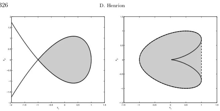
4.1. Rational cubic and quartic. Let
A=
0 0 1
0 1 i
1 i 0
.
Then
F(y) =
y0 0 y1 0 y0+y1 y2
y1 y2 y0
and
p(y) = (y0−y1)(y0+y1)2−y0y22
defines a genus-zero cubic curveP whose connected component containing the origin is the LMI set F(A); see Figure 4.1. With an elimination technique (resultants or Gr¨obner basis with lexicographical ordering), we obtain
q(x) = 4x4 1+ 32x
4 2+ 13x
2 1x
2
2−18x0x1x 2
2+ 4x0x 3 1−27x
2 0x
2 2
−2 −1.5 −1 −0.5 0 0.5 1 1.5 −2
−1.5 −1 −0.5 0 0.5 1 1.5 2
y1
y2
−1.5 −1 −0.5 0 0.5 1 1.5 −1.5
−1 −0.5 0 0.5 1 1.5
x1
[image:5.612.74.431.127.307.2]x2
Fig. 4.1.Left: LMI setF(A)(gray area) delimited by cubicP(black). Right: numerical range
W(A)(gray area, dashed line) convex hull of quarticQ(black solid line).
4.2. Couple of two nested ovals. For
A=
0 2 1 + 2i 0
0 0 1 0
0 i i 0
0 −1 +i i 0
,
the quarticP and its dual octicQboth feature two nested ovals; see Figure 4.2. The
−2 −1.5 −1 −0.5 0 0.5 1 1.5 2 −1.5
−1 −0.5 0 0.5 1 1.5 2 2.5
y1
y2
−2 −1.5 −1 −0.5 0 0.5 1 1.5 2 −2
−1.5 −1 −0.5 0 0.5 1 1.5 2 2.5
x1
[image:5.612.82.430.467.622.2]x2
Fig. 4.2.Left: LMI setF(A)(gray area) delimited by the inner oval of quarticP(black line).
Right: numerical rangeW(A)(gray area) delimited by the outer oval of octicQ(black line).
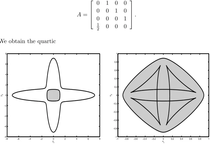
4.3. Cross and star. A computer-generated representation of the numerical range as an envelope curve can be found in [8, Figure 1, p. 139] for
A=
0 1 0 0
0 0 1 0
0 0 0 1
1
2 0 0 0
.
We obtain the quartic
−8 −6 −4 −2 0 2 4 6 8 −8 −6 −4 −2 0 2 4 6 8 y1 y2
[image:6.612.78.431.194.441.2]−1 −0.8 −0.6 −0.4 −0.2 0 0.2 0.4 0.6 0.8 1 −1 −0.8 −0.6 −0.4 −0.2 0 0.2 0.4 0.6 0.8 1 x1 x2
Fig. 4.3.Left: LMI setF(A)(gray area) delimited by the inner oval of quarticP(black line).
Right: numerical range W(A) (gray area) delimited by the outer oval of twelfth-degree Q (black
line).
p(y) = 1 64(64y
4 0−52y
2 0y
2 1−52y
2 0y
2 2+y
4 1+ 34y
2 1y
2 2+y
4 2)
and the dual twelfth-degree polynomial
q(x) = 5184x12
0 −299520x 10 0 x
2
1−299520x 10 0 x
2
2+ 1954576x 8 0x
4 1 +16356256x8
0x 2 1x
2
2+ 1954576x 8 0x
4
2−5375968x 6 0x
6
1−79163552x 6 0x 4 1x 2 2
−79163552x6 0x
2 1x
4
2−5375968x 6 0x
6
2+ 7512049x 4 0x
8
1+ 152829956x 4 0x 6 1x 2 2
−2714586x4 0x
4 1x
4
2+ 152829956x 4 0x
2 1x
6
2+ 7512049x 4 0x
8
2−5290740x 2 0x
10 1
−136066372x2 0x
8 1x
2
2+ 232523512x 2 0x
6 1x
4
2+ 232523512x 2 0x 4 1x 6 2
−136066372x2 0x
2 1x
8
2−5290740x 2 0x
10
2 + 1498176x 12
1 + 46903680x 10 1 x
2 2
−129955904x8 1x
4
2+ 186148096x 6 1x
6
2−129955904x 4 1x
8 2 +46903680x2
1x 10
2 + 1498176x 12 2 ,
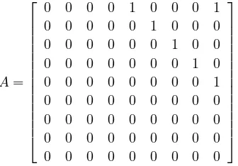
4.4. Decomposition into irreducible factors. Consider the example of [8, Figure 6, p. 144] with
A=
0 0 0 0 1 0 0 0 1
0 0 0 0 0 1 0 0 0
0 0 0 0 0 0 1 0 0
0 0 0 0 0 0 0 1 0
0 0 0 0 0 0 0 0 1
0 0 0 0 0 0 0 0 0
0 0 0 0 0 0 0 0 0
0 0 0 0 0 0 0 0 0
0 0 0 0 0 0 0 0 0
.
The determinant of the trivariate pencil factors as follows:
p(y) = 1 256(4y
3
0−3y0y21−3y0y22+y 3
1+y1y22)(4y02−y 2 1−y
2 2)3
,
which means that the LMI setF(A) is the intersection of a cubic and conic LMI.
y1
y2
−2.5 −2 −1.5 −1 −0.5 0 0.5 1 1.5 2 2.5 3 −2.5 −2 −1.5 −1 −0.5 0 0.5 1 1.5 2 2.5
−0.6 −0.4 −0.2 0 0.2 0.4 0.6 0.8 1 1.2 −1 −0.8 −0.6 −0.4 −0.2 0 0.2 0.4 0.6 0.8 1 x1 x2
Fig. 4.4. Left: LMI set F(A) (gray area) intersection of cubic (black solid line) and conic
(gray line) LMI sets. Right: numerical range W(A)(gray area, black dashed line) convex hull of
the union of a quartic curve (black solid line) and conic curve (gray line).
The dual curveQis the union of the quartic
Q1={x : x
4 0−8x
3
0x1−18x 2 0x
2 1−18x
2 0x
2 2+ 27x
4 1+ 54x
2 1x
2 2+ 27x
4 2= 0}, a cardioid dual to the cubic factor ofp(y), and the conic
Q2={x : x
2 0−4x
2 1−4x
[image:7.612.83.431.393.546.2]a circle dual to the quadratic factor ofp(y). The numerical rangeW(A) is the convex hull of the union of convQ1 and convQ2, which is here the same as convQ1; see Figure 4.4.
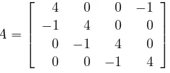
4.5. Polytope. Consider the example of [8, Figure 9, p. 147] with
A=
4 0 0 −1
−1 4 0 0
0 −1 4 0
0 0 −1 4
.
The dual determinant factors into linear terms
p(y) = (y0+ 5y1)(y0+ 3y1)(y0+ 4y1+y2)(y0+ 4y1−y2)
and this generates an unbounded polyhedronF(A) ={y : y0+ 5y1≥0, y0+ 3y1≥ 0, y0+ 4y1+y2≥0, y0+ 4y1−y2≥0}. The dual to curveP is the union of the four
−0.4 −0.35 −0.3 −0.25 −0.2 −0.15 −0.1 −0.5
−0.4 −0.3 −0.2 −0.1 0 0.1 0.2 0.3 0.4 0.5
y1
y2
2.5 3 3.5 4 4.5 5 5.5 −1.5
−1 −0.5 0 0.5 1 1.5
x1
x2
Fig. 4.5. Left: LMI setF(A)(gray area), an unbounded polyhedron. Right: numerical range
W(A)(gray area) convex hull of four vertices.
points (1,5,0), (1,3,0), (1,4,1) and (1,4,−1), and hence, the numerical rangeW(A) is the polytopic convex hull of these four vertices; see Figure 4.5.
5. A problem in statistics. We have seen in Example 4.5 that the numerical range can be polytopic, and this is the case in particular whenAis a normal matrix (i.e., satisfyingA∗A=AA∗); see e.g. [14, Theorem 3] or [8, Theorem 1.4-4].
[image:8.612.82.430.371.524.2]variates following a joint normal distribution; see [4] for an historical account. In its simplest form (called the central case), the result can be stated as follows (in the sequel, we work in the affine planey0= 1):
Theorem 5.1. Let A1 and A2 be Hermitian matrices of size n. Thendet(In+
y1A1+y2A2) = det(In+y1A1) det(In+y2A2)if and only if A1A2= 0.
Proof. If A1A2 = 0, then obviously det(In +y1A1) det(In+y2A2) = det((In+
y1A1)(In+y2A2)) = det(In+y1A1+y2A2+y1y2A1A2) = det(In+y1A1+y2A2). Let us prove the converse statement.
Leta1kanda2krespectively denote the eigenvalues ofA1andA2, fork= 1, . . . , n. Then p(y) = det(In +y1A1+y2A2) = det(In +y1A1) det(In+y2A2) = Qk(1 + y1a1k)
Q
k(1 +y2a2k) factors into linear terms, and we can write p(y) =
Q
k(1 + y1a1k+y2a2k) witha1ka2k = 0 for all k= 1, . . . , n. Geometrically, this means that
the corresponding numerical rangeW(A) forA=A1+iA2is a rectangle with vertices (minkak,minkbk), (minkak,maxkbk), (maxkak,minkbk) and (maxkak,maxkbk).
Following the terminology of [15],A1andA2satisfy property L sincey1A1+y2A2 has eigenvalues y1a1k+y2a2k fork = 1, . . . , n. By [15, Theorem 2], it follows that A1A2 =A2A1, and hence that the two matrices are simultaneously diagonalisable: there exists a unitary matrixU such thatU∗
A1U = diagka1kandU
∗
A2U = diagka2k.
Since a1ka2k = 0 for all k, we have
P
ka1ka2k =U
∗
A1U U∗A2U =U∗A1A2U = 0, and hence,A1A2= 0.
6. Conclusion. The geometry of the numerical range, studied to a large extent by Kippenhahn in [14] – see [20] for an English translation with comments and correc-tions – is revisited here from the perspective of semidefinite programming duality. In contrast with previous studies of the geometry of the numerical range, based on dif-ferential topology [13], it is namely noticed that the numerical range is a semidefinite representable set, an affine projection of the semidefinite cone, whereas its geometric dual is an LMI set, an affine section of the semidefinite cone. The boundaries of both primal and dual sets are components of algebraic plane curves explicitly formulated as locii of determinants of Hermitian pencils. The geometry of the numerical range is therefore the geometry of (planar sections and projections of) the semidefinite cone, and hence every study of this cone is also relevant to the study of the numerical range.
men-tioned in [12, Section 1.8]. In this context, it would be interesting to derive condi-tions on three matrices A1, A2, A3 ensuring that det(In+y1A1+y2A2+y3A3) = det(In+y1A1) det(In +y2A2) det(In+y3A3). Another extension of the numerical range to matrix polynomials (including matrix pencils) was carried out in [2], also using algebraic geometric considerations, and it could be interesting to study semidef-inite representations of convex hulls of these numerical ranges.
The inverse problem of finding a matrix given its numerical range (as the convex hull of a given algebraic curve) seems to be difficult. In a sense, it is dual to the problem of finding a symmetric (or Hermitian) definite linear determinantal represen-tation of a trivariate form: givenp(y) satisfying a real zero (hyperbolicity) condition, find Hermitian matrices Ak such that p(y) = det(PkykAk), with A0 positive defi-nite. Explicit formulas are described in [9] based on transcendental theta functions and Riemann surface theory, and the case of curves{y : p(y) = 0} of genus zero is settled in [10] using B´ezoutians. A more direct and computationally viable approach in the positive genus case is still missing, and one may wonder whether the geometry of the dual object, namely, the numerical range conv{x : q(x) = 0}, could help in this context.
Acknowledgment. The author is grateful to Leiba Rodman for his suggestion of studying rigid convexity of the numerical range. This work also benefited from technical advice by Jean-Baptiste Hiriart-Urruty who recalled Theorem 5.1 in the September 2007 issue of the MODE newsletter of SMAI (French society for applied and industrial mathematics) and provided reference [4]. Finally, references [2, 13] were brought to the author’s attention by an anonymous referee, who also pointed out several errors and inaccuracies in previous versions of this paper.
REFERENCES
[1] A. Ben-Tal and A. Nemirovski.Lectures on Modern Convex Optimization. SIAM, Philadelphia, 2001.
[2] M.T. Chien, H. Nakazato, and P. Psarrakos. Point equation of the boudary of the numerical range of a matrix polynomial. Linear Algebra and its Applications, 347:205–217, 2002. [3] C.C. Cowen and E. Harel.An effective algorithm for computing the numerical range. Technical
report, Department of Mathematics, Purdue University, 1995.
[4] M.F. Driscoll and W.R. Gundberg Jr. A history of the development of Craig’s theorem. The
American Statistician, 40(1):65–70, 1986.
[5] M.K.H. Fan and A.L. Tits. On the generalized numerical range.Linear and Multilinear Algebra, 21(3):313–320, 1987.
[6] M. Fiedler. Geometry of the numerical range of matrices. Linear Algebra and its Applications, 37:81–96, 1981.
[7] I.M. Gelfand, M.M. Kapranov, and A.V. Zelevinsky. Discriminants, Resultants and
[8] K.E. Gustafsson and D.K.M. Rao. Numerical Range: the Field of Values of Linear Operators
and Matrices. Springer, Berlin, 1997.
[9] J.W. Helton and V. Vinnikov. Linear matrix inequality representation of sets.Communications
in Pure and Applied Mathematics, 60(5):654–674, 2007.
[10] D. Henrion. Detecting rigid convexity of bivariate polynomials. Linear Algebra and its
Appli-cations, 432:1218–1233, 2010.
[11] N.J. Higham. The Matrix Computation Toolbox, Version 1.2, 2002.
[12] R.A. Horn and C.R. Johnson. Topics in Matrix Analysis. Cambridge University Press, Cam-bridge, 1991.
[13] E.A. Jonckheere, F. Ahmad, and E. Gutkin. Differential topology of numerical range. Linear
Algebra and its Applications, 279:227–254, 1998.
[14] R. Kippenhahn. ¨Uber den Wertevorrat einer Matrix.Mathematische Nachrichten, 6(3/4):193– 228, 1951.
[15] T.S. Motzkin and O. Taussky. Pairs of matrices with property L.Transactions of the American
Mathematical Society, 73(1):108–114, 1952.
[16] F.D. Murnaghan. On the field of values of a square matrix.Proceedings of the National Academy
of Sciences of the United States of America, 18(3):246–248, 1932.
[17] A. Packard and J. Doyle. The complex structured singular value. Automatica, 29(1):71–109, 1993.
[18] J. Stolfi. Primitives for Computational Geometry. PhD Thesis, Department of Computer
Science, Stanford University, California, 1988
[19] R.J. Walker.Algebraic Curves. Princeton University Press, Princeton, 1950.
[20] P.F. Zachlin and M.E. Hochstenbach. On the numerical range of a matrix. Linear and
Multi-linear Algebra, 56(1/2):185–225, 2008. English translation with comments and corrections