Full Terms & Conditions of access and use can be found at
http://www.tandfonline.com/action/journalInformation?journalCode=ubes20
Download by: [Universitas Maritim Raja Ali Haji] Date: 12 January 2016, At: 17:25
Journal of Business & Economic Statistics
ISSN: 0735-0015 (Print) 1537-2707 (Online) Journal homepage: http://www.tandfonline.com/loi/ubes20
Weak Instrument Robust Tests in GMM and the
New Keynesian Phillips Curve
Frank Kleibergen & Sophocles Mavroeidis
To cite this article: Frank Kleibergen & Sophocles Mavroeidis (2009) Weak Instrument Robust
Tests in GMM and the New Keynesian Phillips Curve, Journal of Business & Economic Statistics, 27:3, 293-311, DOI: 10.1198/jbes.2009.08280
To link to this article: http://dx.doi.org/10.1198/jbes.2009.08280
Published online: 01 Jan 2012.
Submit your article to this journal
Article views: 456
View related articles
Weak Instrument Robust Tests in GMM and
the New Keynesian Phillips Curve
Frank K
LEIBERGENand Sophocles M
AVROEIDISDepartment of Economics, Brown University, 64 Waterman Street, Providence, RI 02912 (Frank_Kleibergen@brown.edu;Sophocles_Mavroeidis@brown.edu)
We discuss weak instrument robust statistics in GMM for testing hypotheses on the full parameter vec-tor or on subsets of the parameters. We use these test procedures to reexamine the evidence on the new Keynesian Phillips curve model. We find that U.S. postwar data are consistent with the view that infla-tion dynamics are predominantly forward-looking, but we cannot rule out the presence of considerable backward-looking dynamics. Moreover, the Phillips curve has become flatter recently, and this is an im-portant factor contributing to its weak identification.
KEY WORDS: Identification; Power of tests; Size distortion; Structual breaks.
1. INTRODUCTION
The new Keynesian Phillips curve (NKPC) is a forward-looking model of inflation dynamics, according to which short-run dynamics in inflation are driven by the expected discounted stream of real marginal costs. Researchers often use a specifica-tion that includes both forward-looking and backward-looking dynamics; see, for example,Buiter and Jewitt (1989), Fuhrer and Moore (1995), andGalí and Gertler (1999):
πt=λxt+γfEt(πt+1)+γbπt−1+ut, (1)
whereπtdenotes inflation,xtis some proxy for marginal costs, Et denotes the expectation conditional on information up to
timet, andut is an unobserved cost-push shock. This model
can be derived from microfoundations in a dynamic general equilibrium framework with price stickiness, a la Calvo (1983), and indexation, seeWoodford (2003). Variants of Equation (1) appear in many studies on macroeconomic dynamics and mon-etary policy; see, for example,Lubik and Schorfheide (2004) and Christiano, Eichenbaum, and Evans (2005). Equation (1) is usually referred to as the “semistructural” specification corre-sponding to a deeper microfounded structural model. The var-ious structural specifications proposed in the literature share essentially the same semistructural form, but their underlying deep parameters, which are functions of λ, γf, and γb,
dif-fer. Hence, we choose to focus our discussion mainly on the semistructural specification, which is more general, but we also present empirical results for a popular structural version of the model.
In a seminal paper,Galí and Gertler (1999)estimated a ver-sion of this model in which the forcing variablext is the labor
share and the parameters λ, γf, γb are functions of three key
structural parameters: the fraction of backward-looking price-setters, the average duration an individual price is fixed (the de-gree of price stickiness), and a discount factor. Using postwar data on the U.S.,Galí and Gertler (1999)reported that real mar-ginal costs are statistically significant and inflation dynamics are predominantly forward-looking. They foundγbto be
statis-tically significant but quantitatively small relative toγf.
Several authors have argued that the above results are unre-liable because they are derived using methods that are not
ro-bust to identification problems, also known as weak instrument problems; seeCanova and Sala (2009),Mavroeidis (2005), and Nason and Smith (2008). As we explain below, weak instru-ment problems arise if marginal costs have limited dynamics or if their coefficient is close to zero, that is, when the NKPC is flat, since in those cases the exogenous variation in inflation forecasts is limited. Moreover, the weak instruments literature (cf. Stock, Wright, and Yogo2002; Dufour2003; Andrews and Stock2005; and Kleibergen2007) has shown that using con-ventional inference methods after pretesting for identification is both unreliable and unnecessary. It is unreliable because the size of such two-step testing procedures cannot be controlled. It is unnecessary because there are identification robust methods that are as powerful as the nonrobust methods when instruments are strong and more powerful than the aforementioned two-step procedures when instruments are weak. For example, we show that when the instruments are weak, the commonly used pretest rule advocated by Stock and Yogo (2005)—to only use two-stage least-squares t-statistics when the first-stage F-statistic exceeds ten—has less power than the identification robust sta-tistic of Anderson and Rubin (1949).
Unfortunately, the use of identification robust methods has not yet become the norm in this literature. To the best of our knowledge, the studies that did use identification robust meth-ods areMa (2002),Nason and Smith (2008), Dufour, Khalaf, and Kichian (2006), andMartins and Gabriel (2006), and their results suggest that the NKPC is weakly identified. In particular, they could not find evidence in favor of the view that forward-looking dynamics are dominant, or that the labor share is a sig-nificant driver of inflation. These results seem to confirm the criticism ofMavroeidis (2005)regarding the poor identifiabil-ity of the NKPC.
In this article, we discuss the various identification robust methods that can be used to conduct inference on the parame-ters of the NKPC, with particular emphasis on the problem of inference on subsets of the parameters. Our discussion of the
© 2009American Statistical Association Journal of Business & Economic Statistics
July 2009, Vol. 27, No. 3 DOI:10.1198/jbes.2009.08280
293
theoretical econometrics literature and the results of the Monte Carlo simulations that we conducted for the NKPC lead us to recommend as the preferred method of inference the general-ized method of moments (GMM) extension of the conditional likelihood ratio (CLR) statistic. The CLR statistic was proposed by Moreira (2003) for the linear instrumental variables regres-sion model with one included endogenous variable and it was later extended to GMM by Kleibergen (2005). We refer to this extension as the MQLR statistic. The MQLR is at least as pow-erful as any of the other tests and yields the smallest confidence sets in our empirical application. We also provide an efficient method for computing a version of the MQLR statistic that has some appealing numerical properties.
Our empirical analysis is based on quarterly postwar U.S. data from 1960 to 2007. We obtain one- and two-dimensional confidence sets derived by inverting each of the identification robust statistics for the key parameters of the NKPC and our results for the full sample can be summarized as follows. In accordance with Galí and Gertler (1999), we find evidence that forward-looking dynamics in inflation are statistically sig-nificant and that they dominate backward-looking dynamics. However, the confidence intervals are so wide that they are consistent both with no backward-looking dynamics and very substantial backward-looking behavior. Moreover, we cannot reject the null hypothesis that the coefficient on the labor share is zero. We also test the deeper structural parameters in the model of Galí and Gertler (1999), which characterize the de-gree of price stickiness and the fraction of backward-looking price setters. With regards to price stickiness, the 95% confi-dence interval, though unbounded from above, is still informa-tive because it suggests that prices remain fixed for a least two quarters, thus uncovering evidence of significant price rigidity. However, regarding the fraction of backward-looking price set-ters, the 95% confidence interval is very wide, suggesting that the data are consistent both with the view that price-setting be-havior is purely forward-looking and with the opposite view that it is predominantly backward-looking.
Finally, we conduct an identification robust structural stabil-ity test proposed by Caner (2007) and find evidence of instabil-ity before 1984, but no such evidence thereafter. This shows that the model is not immune to theLucas (1976)critique. When we split the sample in half to pre- and post-1984 periods, we find that the slope of the NKPC is markedly smaller in the second half of the sample, lending some support to the view that the Phillips curve is now flatter than it used to be. This finding may have useful implications for the conduct of monetary policy.
The structure of the article is as follows. In Section 2, we introduce the model and discuss the main identification issues. Section3presents the relevant econometric theory for the iden-tification robust tests. Monte Carlo simulations on the size and power of those tests for the NKPC are reported in Section 4 and the results of the empirical analysis are given in Section5. Section6discusses some directions for future research and Sec-tion7concludes. Analytical derivations are provided in an Ap-pendixat the end.
Throughout the article, we use the following notation:Im is
the m×m identity matrix, PA=A(A′A)−1A′ for a full rank n×mmatrixAandMA=In−PA. Furthermore, “
p
→” stands for convergence in probability, “→d” for convergence in
distrib-ution,Eis the expectation operator, andEtdenotes expectations
conditional on information available at timet.
2. IDENTIFICATION OF THE NEW KEYNESIAN PHILLIPS CURVE
The parameters of the NKPC model are typically estimated using a limited information method that replaces the unob-served termEt(πt+1)in Equation (1) byπt+1−ηt+1, where ηt is the one-step-ahead forecast error inπt, to obtain the
es-timable equation
πt=λxt+γfπt+1+γbπt−1+et, (2)
withet=ut−γfηt+1. The assumptionEt−1(ut)=0 implies that Et−1(et)=0, so Equation (2) can be estimated by GMM
us-ing any predetermined variablesZtas instruments. The moment
conditions are given by E(ft(θ ))=0, where ft(θ )=Zt(πt − λxt−γfπt+1−γbπt−1) and θ=(λ, γf, γb). Note that since et is not adapted to the information at timet, it does not
fol-low from the above assumptions thatE(etet−1)=0 and hence
et may exhibit first-order autocorrelation without
contradict-ing the model. Moreover,etmay also be heteroscedastic. Thus
Equation (2) does not fit into the framework of the linear instru-mental variables (IV) regression model with independently and identically distributed (iid) data. Nonetheless, the tools used to study identification in the linear IV regression model can be used to discuss the relevant identification issues for the NKPC. We first consider the rank condition for identification of the parameters in (2). The parametersθ are identified if the Jaco-bian of the moment conditionsE(∂ft(θ )
∂θ′ )is of full rank.
Equa-tion (2) has two endogenous regressors, πt+1 andxt, and one
exogenous regressorπt−1. If1πt−1+2Z2,tdenotes the
lin-ear projection of the endogenous regressors(πt+1,xt)on the
instrumentsZt=(πt−1,Z2′,t)′, the rank condition for identifica-tion is that the rank of2is equal to two sinceπt−1is included as an exogenous regressor in Equation (2).
To study the rank condition for identification, we need to model the reduced-form dynamics of πt and xt. This can be
done by postulating a model for the forcing variable, xt, and
solving the resulting system of equations to obtain the restricted reduced-form model for the joint law of motion of(πt,xt). This
enables us to express the coefficient matrix2in the projection of the endogenous regressors(πt+1,xt)on the instrumentsZ2,t
as a function of the structural parameters. Because the rank con-dition is intractable in general, see Pesaran (1987, chapter 6), it is instructive to study a leading special case in which analytical derivations are straightforward, and which suffices to provide the main insights into the identification problems.
Consider the purely forward-looking version of model (1) with γb=0 and assume that xt is stationary and follows a
second-order autoregression. The complete system is given by the equations:
πt=λxt+γfEt(πt+1)+ut, (3) xt=ρ1xt−1+ρ2xt−2+vt. (4)
Solving Equation (3) forward, we obtain
πt=λ
∞
j=0
γfjEt(xt+j)+ut=α0xt+α1xt−1+ut, (5)
withα0=λ/[1−γf(ρ1+γfρ2)]andα1=λγfρ2/[1−γf(ρ1+ γfρ2)]. The solution can be verified by computing Et(πt+1), substituting into the model (1) and matching the coefficients onxt andxt−1 in the resulting equation to α0 andα1 in (5). Substituting forxtin (5) using (4), and evaluating the resulting
expression at timet+1, we obtain the first-stage regression for the endogenous regressorsπt+1,xt
Et−1(πt+1)
Et−1(xt)
=
α0((ρ1+ρ2γf)ρ1+ρ2) α0(ρ1+ρ2γf)ρ2
ρ1 ρ2
×
xt−1
xt−2
Zt
. (6)
It is then straightforward to show that the determinant of the coefficient matrixin the above expression is proportional to α0ρ22, and hence, sinceα0is proportional toλ, the rank condi-tion for identificacondi-tion is satisfied if and only ifλ=0 andρ2=0. Thus, identification requires the presence of second-order dy-namics and thatλexceeds zero (since economic theory implies λ≥0).
The rank condition is, however, not sufficient for reliable es-timation and inference because of the problem of weak instru-ments; see, for example,Stock, Wright, and Yogo (2002). Even when the rank condition is satisfied, instruments can be weak for a wide range of empirically relevant values of the parame-ters. Loosely speaking, instruments are weak whenever there is a linear combination of the endogenous regressors whose corre-lation with the instruments is small relative to the sample size. More precisely, the strength of the instruments is characterized in linear IV regression models by a unitless measure known as the concentration parameter; see, for example, Phillips (1983) and Rothenberg (1984). The concentration parameter is a mea-sure of the variation of the endogenous regressors that is ex-plained by the instruments after controlling for any exogenous regressors relative to the variance of the residuals in the first-stage regression, that is, a multivariate signal-to-noise ratio in the first-stage regression. For the first-stage regression given in Equation (6), the concentration parameter can be written as T−VV1/2′E(ZtZ′t)−
1/2
VV , where VV is the variance of
first-stage regression residuals andT is the sample size. This is a symmetric positive semidefinite matrix whose dimension is equal to the number of endogenous regressors. The inter-pretation of the concentration parameter is most easily given in a model with a single endogenous regressor in terms of the so-called first-stageF-statistic that tests the rank condition for identification. Under the null hypothesis of no identification, that is, when the instruments are completely irrelevant, the ex-pected value of the first-stage F-statistic is equal to 1, while under the alternative it is greater than 1. The concentration pa-rameter, divided by the number of instruments,μ2/k, is then approximately equal toE(F)−1. In the case ofmendogenous regressors, the strength of the instruments can be measured by the smallest eigenvalue of the concentration matrix, which we shall also denote byμ2, to economize on notation.
Even in the above simple model, which has only two endoge-nous regressors, πt+1 and xt, the analytical derivation of the
smallest eigenvalue of the concentration matrix,μ2, is imprac-tical. Thus, we shall consider a special case in which the model has a single endogenous regressor, so that μ2 can be derived analytically. This special case suffices for the points we raise in this section. For the Monte Carlo experiments reported in Sec-tion4, where we consider the general case with two endogenous regressors, the concentration parameter is computed by simula-tion. This special case arises when we assume thatE(vtut)= E(xtut)=0, so that the regressorxt in Equation (3) becomes
exogenous, and the only endogenous regressor isπt+1. Hence, the first-stage regression is given byEt(πt+1). From the law of motion ofπt,xt given by Equations (5) and (4), we obtain that Et(πt+1)=α0Et(xt+1)+α1xt=α0ρ1xt+α0ρ2xt−1+α1xtand
hence the first-stage regression can be written equivalently as
πt+1=(α0ρ1+α1)xt+α0ρ2xt−1+ηt+1, (7) whereηt=ut+α0vtis the one-step innovation inπt. To
sim-plify the derivations, assume further thatut,vt are jointly
nor-mally distributed and homoscedastic. SinceE(utvt)=0, it
fol-lows thatE(vtηt)≡ρηvσvση=α0σv2, orα0=ρηvση/σv, where ση2=E(ηt2),σv2=E(vt2), andρηv=E(ηtvt)/(σvση). Recall that xt is the exogenous regressor, andxt−1is the additional (opti-mal) instrument. The parameter that governs identification is therefore the coefficient of xt−1 in the first-stage regression (7), that is,α0ρ2 or ρηvρ2ση/σv. The expression of the
con-centration parameter corresponds to T(α0ρ2)2E(x2t−1|xt)/ση2.
Now, since xt and xt−1 are jointly normal random variables with zero means, it follows thatE(x2t−1|xt)=var(xt−1|xt)is
in-dependent ofxt and is equal toσv2/(1−ρ22). SinceE(xt)=0,
var(xt−1|xt)=E(x2t−1)−E(xtxt−1)2/E(x2t)=σv2(1−ρ2)/((1− ρ22)(1−ρ2))=σv2/(1−ρ22), whereρis the first autocorrelation ofxt. Hence, the concentration parameterμ2is:
μ2=Tρ 2 2ρη2v
1−ρ22 =
Tλ2ρ22σv2
(1−ρ22)(1−γf(ρ1+γfρ2))2ση2
, (8)
sinceλ=ρηvση/σv(1−γf(ρ1+γfρ2)).
It is interesting to note that, for a fixed value ofλ, the con-centration parameter varies nonmonotonically withγf and this
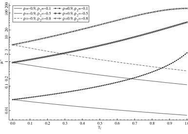
has implications for the power of a test ofH0:γf =γf,0against an alternative H1:γf =γf,1. To illustrate this, Figure 1 plots μ2as a function ofγf whenλ=0.5, for different values ofρ,
the first-order autocorrelation coefficient ofxt, andρ2. When γf,0=0.5, Figure 1 shows that μ2 is increasing in γf when ρ >0, and decreasing in γf when ρ <0. Thus, whenρ >0,
tests of H0:γf,0=0.5 have more power against alternatives
H1:γf =γf,1 for which γf,1 >0.5 than against alternatives
H1:γf =γf,1, for whichγf,1<0.5 and vice versa whenρ <0. Depending on the value ofρ andρ2, the variation in the qual-ity of identification under the alternative can be very large. For example, whenρ=0.9 andρ2= −0.8, the concentration para-meter goes from rather low (about 5) forγf =0, to very high
(150) forγf =1. This fact has implications for the study of the
power function of tests onγf. We explore this issue further in
Section4below.
The above discussion focused on a special case of the model in which the concentration parameter is analytically tractable.
Figure 1. Concentration parameterμ2as a function ofγf for different values ofρandρ2, holdingλfixed at 0.5 andση=3.
In more complicated situations, the concentration parameter can be computed numerically.Mavroeidis (2005) computed it for the model given by Equations (2) and (4) for different values of the parametersλ,ρ2and the relative size of the shocksσv/σu
and found that it is very small (in the order of 10−4) for typical values of the parameters reported in the literature. The concen-tration parameter remains small except for extreme departures of the parametersρ2,λ, andσv/σufrom their estimated values.
This shows that we should avoid doing inference on the para-meters of the NKPC model using procedures that are not robust to weak instruments, since they give unreliable results.
3. WEAK INSTRUMENT ROBUST TESTS FOR THE NKPC
We employ weak instrument robust tests to conduct inference on the parameters of the NKPC model. These tests are defined for GMM so we start their discussion with a brief outline of Hansen’s (1982) GMM.
GMM provides a framework for inference on a p -dimen-sional vector of parametersθfor which thek-dimensional mo-ment equation
E(ft(θ ))=0, t=1, . . . ,T, (9)
holds. For the NKPC, the moment vector reads
ft(θ )=Zt(πt−λxt−γfπt+1−γbπt−1) (10) as defined in Equations (1)–(2). We assume that the moment equation in (9) is uniquely satisfied at θ0. The weak instru-ment robust statistics are based on the objective function for the continuous updating estimator (CUE) ofHansen, Heaton, and Yaron (1996):
Q(θ )=TfT(θ )′Vˆff(θ )−1fT(θ ), (11)
withfT(θ )=T1 Tt=1ft(θ ). Thek×k-dimensional covariance
matrix estimatorVˆff(θ )that we use in (11) is a consistent
es-timator of the covariance matrixVff(θ )of the moment vector.
Besides the moment vectorft(θ ), we use its derivative with
re-spect toθ, which, for the NKPC model, reads
qt(θ )=vec
∂ft(θ )
∂θ′
= −
x
t πt+1 πt−1
⊗Zt
, (12)
andqT(θ )=T1 Tt=1qt(θ ). To obtain the limiting distributions
of the weak instrument robust statistics, we assume that the sample average of the moment vector and its derivative follow a normal random process; see Kleibergen and Mavroeidis (2008).
Assumption 1. The large sample behavior off¯t(θ )=ft(θ )− E(ft(θ ))andq¯t(θ )=qt(θ )−E(qt(θ ))satisfies
ψT(θ )≡
1
√
T T
t=1 f¯
t(θ )
¯
qt(θ )
d
→
ψ
f(θ ) ψθ(θ )
, (13)
whereψ (θ )=ψf(θ )
ψθ(θ )
is ak(p+1)-dimensional Normal distrib-uted random process with mean zero and positive semidefinite
k(p+1)×k(p+1)-dimensional covariance matrix
V(θ )= V
ff(θ ) Vfθ(θ ) Vθf(θ ) Vθ θ(θ )
(14)
withVθf(θ )=Vfθ(θ )′=(Vθf,1(θ )′ · · · Vθf,p(θ )′)′,Vθ θ(θ )= Vθ θ,ij(θ ),i,j=1, . . . ,p, andVff(θ ),Vθf,i(θ ),Vθ θ,ij(θ )arek×k
-dimensional matrices fori,j=1, . . . ,p, and
V(θ )= lim
T→∞var
√
T
fT(θ ) qT(θ )
. (15)
Equation (12) shows thatqt(θ )does not depend onθ.
More-over, sinceft(θ )is linear inθ, Assumption1is basically just a
central limit theorem forft(θ0)andqt(θ0)that holds under mild conditions. For example, sufficient conditions for Assumption1 are that therth moments of the absolute values of ¯ft(θ0)and
¯
qt(θ0)are finite for some r>2 and theϕ orα-mixing coeffi-cients off¯t(θ0)andq¯t(θ0)are of sizes/(s−1)withs>1; see, for example, White (1984, theorem 5.19).
Assumption1 differs from the traditional assumptions that are made to obtain the limiting distributions of estimators and test statistics in GMM; see for example, Hansen (1982) and Newey and McFadden (1994). These assumptions consist of a normal random process assumption for the limiting behavior of √1
T T
t=1f¯t(θ ) and a full rank assumption for the expected
value of the Jacobian,J(θ )=E(limT→∞∂θ∂′fT(θ )). Since
As-sumption1 also makes a normal random process assumption for the limiting behavior of √1
T T
t=1f¯t(θ ), the difference
be-tween the traditional assumption and Assumption1 is that the full rank assumption forJ(θ )is replaced by a normal random process assumption for the limiting behavior of√1
T T t=1q¯t(θ ).
Sinceq¯t(θ )is a mean zero random variable, the normal random
process assumption for its scaled sum is, as explained above, a mild assumption. The full rank assumption ofJ(θ )is, how-ever, an assumption on a nuisance parameter and therefore dif-ficult to verify. The limiting distributions of statistics that result under Assumption1therefore hold more generally than the lim-iting distributions of statistics that result under the traditional assumptions.
To estimate the covariance matrix, we use the covari-ance matrix estimator Vˆ(θ ), which consists of Vˆff(θ ):k×k,
ˆ
Vθf(θ ):kθ×k, andVˆθ θ(θ ):kθ×kθ,kθ =pk. We assume that
the covariance matrix estimator is a consistent one for every value ofθ. Because of the specific functional form of the deriv-ative (12) for the NKPC, the assumption on the convergence of the derivative ofVˆff(θ )that is made in Kleibergen (2005) is
automatically satisfied.
The derivative estimatorqT(θ ) is correlated with the
aver-age moment vector fT(θ )since Vθf(θ )=0. The weak
instru-ment robust statistics therefore use an alternative estimator of the derivative of the unconditional expectation of the Jacobian,
ˆ
DT(θ0)=[q1,T(θ0)− ˆVθf,1(θ0)Vˆff(θ0)−1fT(θ0) · · ·
qp,T(θ0)− ˆVθf,p(θ0)Vˆff(θ0)−1fT(θ0)], (16) whereVˆθf,i(θ )arek×k-dimensional estimators of the
covari-ance matrices Vθf,i(θ ),i=1, . . . ,p,Vˆθf(θ )=(Vˆθf,1(θ )′ · · ·
ˆ
Vθf,p(θ )′)′, and qT(θ0) = (q′1,T(θ0) · · · q′p,T(θ0))′. Since
ˆ
Vθf,j(θ0)Vˆff(θ0)−1fT(θ0) is the projection of qj,T(θ0) onto
fT(θ0), for j=1, . . . ,p, it holds that DˆT(θ0) is asymptoti-cally uncorrelated withfT(θ0). Thus, when Assumption1 and
H0:θ=θ0hold,DˆT(θ0)is an estimator of the expected value of the Jacobian, which is independent of the average moment vectorfT(θ0)in large samples.
The expression of the CUE objective function in (11) is such that both the average moment vectorfT(θ )and the covariance
matrix estimatorVˆff(θ )are functions ofθ. In the construction of
the derivative of the CUE objective function with respect toθ, the derivative ofVˆff(θ ) is typically ignored because it is of a
lower order in the sample size when the Jacobian has a full rank value, that is, when the instruments are strong. However, when the instruments are weak, the contribution of the derivative of
ˆ
Vff(θ )with respect toθ to the derivative of the CUE objective
function is no longer negligible and hence the expression that ignores it is incorrect. When we incorporate the derivatives of bothfT(θ ) andVˆff(θ ) with respect to θ, the derivative of the
CUE objective function with respect toθreads (see Kleibergen 2005),
1 2
∂Q(θ )
∂θ′ =TfT(θ ) ′Vˆ
ff(θ )−1DˆT(θ ). (17)
The independence offT(θ )andDˆT(θ )in large samples and
the property that the derivative of the CUE objective function equals the (weighted) product offT(θ )andDˆT(θ )in (17)
im-ply that we can construct statistics based on the CUE objective function whose limiting distributions are robust to weak instru-ments. We provide the definition of four of these statistics. The first is theS-statistic of Stock and Wright (2000), which equals the CUE objective function (11). The second statistic is a score or Lagrange Multiplier statistic that is equal to a quadratic form of (17) with respect to(DˆT(θ )′Vˆff(θ )−1DˆT(θ ))−1, which can be
considered as the inverse of the (conditional) information ma-trix; see Kleibergen (2007). We refer to this statistic as the KLM statistic. The third statistic is an overidentification statistic that equals the difference between theSand KLM statistics. We re-fer to this statistic as the JKLM statistic. The fourth and last statistic is an extension of the conditional likelihood ratio sta-tistic of Moreira (2003) towards GMM; see Kleibergen (2005). We refer to this statistic as the MQLR statistic.
Definition 1. Let θ=(α′...β′)′, withα andβ being pα and pβ-dimensional vectors, respectively, such thatpα+pβ=p. To
simplify the notation, we denoteQ(θ )evaluated atθ=(α′...β′)′ by Q(α, β) and use the same notation for all other functions ofθ. Four statistics that test the hypothesisH0:β=β0are:
1. The subsetS-statistic of Stock and Wright (2000):
S(β0)=Q(α(β˜ 0), β0), (18) whereα(β˜ 0)is the CUE ofαgiven thatβ=β0.
2. The subset KLM statistic of Kleibergen (2005):
KLM(β0)=fT(α(β˜ 0), β0)′Vˆff(α(β˜ 0), β0)−1/2
×PVˆ
ff(α(β˜ 0),β0)−1/2DˆT(α(β˜ 0),β0)
× ˆVff(α(β˜ 0), β0)−1/2fT(α(β˜ 0), β0). (19) 3. The subset JKLM overidentification statistic:
JKLM(β0)=S(β0)−KLM(β0). (20) 4. The subset extension of the conditional likelihood ratio
statistic of Moreira (2003) applied in a GMM setting:
MQLR(β0)
=1
2
KLM(β0)+JKLM(β0)−rk(β0)
+{KLM(β0)+JKLM(β0)+rk(β0)}2
−4 JKLM(β0)rk(β0) 1/2
, (21)
whererk(β0)is a statistic that tests for a lower rank value
The specifications of the weak instrument robust statistics in Definition1apply both to tests of hypotheses on subsets of the parameters and the full vector of parameters, in which caseβ coincides withθandαdrops out of the expressions.
It is useful to view therk(β0)statistic in the expression of the MQLR statistic [see Equation (22)] as the result of mini-mizing another CUE objective function. Specifically, define the
k×(p+1)matrixFT as
and letWˆ denote a consistent estimator of the asymptotic vari-ance of √Tvec(FT). Then, ft(θ ) in (10) can be alternatively
Ik]. Hence, the CUE objective function in (11) can be
speci-fied in the same form as the minimand on the right-hand side of therk(β0)statistic in (22), and sork(β0)results from mini-mizing another CUE GMM objective function. Conversely, the CUE objective function (11) corresponds to a statistic that tests that the rank of thek×(p+1)matrixE(limT→∞FT)is equal
top. A more detailed explanation of this point is given in the Appendix.
The specification ofrk(β0)in (22) is an alternative specifi-cation of the Cragg and Donald (1997) rank statistic that tests whether the rank of the Jacobian evaluated at (α(β˜ 0), β0) is equal top−1. We evaluate the Jacobian at(α(β˜ 0), β0)since we use an estimate ofα0,α(β˜ 0)in the expressions of the dif-ferent statistics in Definition1. Of course, when the moment conditions are linear, as is the case for the NKPC model,J(θ ) is independent ofθ, soα(β˜ 0)does not appear in the expression of the Jacobian. The specification in (22) is more attractive than the one originally proposed by Cragg and Donald (1997) since it requires optimization over a(p−1)-dimensional space while the statistic proposed by Cragg and Donald (1997) requires op-timization over a(k+1)(p−1)-dimensional space. Other rank statistics, like those proposed by Lewbel (1991), Robin and Smith (2000), or Kleibergen and Paap (2006), can also be used for rk(β0)but the specification in (22) is convenient since it guarantees thatrk(β) >˜ S(β)˜ , which is necessary for MQLR(β) to be equal to zero at the CUE; see Kleibergen (2007). Both the equality of (22) to the Cragg and Donald (1997) rank statistic
and thatS(β) <˜ rk(β)˜ are proven in theAppendix. Whenp=1, the definition ofrk(β0)is unambiguous and reads
rk(β0)=TDˆT(β0)′Vˆθ θ·f(β0)−1DˆT(β0). (24) The robustness of the statistics stated in Definition1to weak instruments was until recently only guaranteed for tests on the full parameter vector; see, for example, Stock and Wright (2000), Kleibergen (2002,2005), and Moreira (2003). Recent results by Kleibergen (2008) and Kleibergen and Mavroeidis (2008) show that the robustness to weak instruments extends to tests on a subset of the parameters when the unrestricted pa-rameters are estimated using the CUE under the hypothesis of interest.
To get the intuition behind the above result, which is formally stated in Theorem1below, it is useful to interpret the CUE ob-jective function as a measure of the distance of a matrix from a reduced rank value. We just showed that the CUE objective function corresponds to a statistic that tests that the rank of the matrixE(limT→∞FT)[see Equation (23)] is reduced by one,
that is, it is equal top. Indeed, when the moment conditions hold, the rank of the above matrix is at mostp. Now, when the parameterαthat is partialled out is well identified, the firstpα
columns of the Jacobian of the moment conditionsJ(θ ) consti-tute a full rank matrix. The (conditional) limiting distributions of the subset statistics for the parameterβ are then equal to those of the corresponding statistics that test a hypothesis on the full parameter vector after appropriately correcting the degrees of freedom parameter of the (conditional) limiting distributions. In contrast, whenαis not well identified, the firstpα columns
of the Jacobian are relatively close to a reduced rank value. But sinceJ(θ )is a submatrix of the matrixFT that appears in the
CUE objective function, weak identification ofαimplies that
FT will be close to a matrix whose rank is reduced even
fur-ther, relative to the case whenαis well identified. This explains why the limiting distribution of the CUE objective function for weakly identified values of α is bounded from above by the limiting distribution that results for well-identified values ofα. The CUE objective function corresponds to theS-statistic and, since the subset statistics in Definition1 are all based on the
S-statistic, the above argument extends to the other subset statis-tics as well; see Kleibergen and Mavroeidis (2008). The (condi-tional) limiting distributions of the subset statistics under well-identified values ofα therefore provide upper bounds on the (conditional) limiting distributions in general.
Theorem 1. Under Assumption1andH0:β=β0, the (con-ditional) limiting distributions of the subset S, KLM, JKLM, and MQLR statistics given in Definition1are such that
S(β0)
where “
a” indicates that the limiting distribution of the statistic
on the left-hand side of the
a sign is bounded by the random
variable on the right-hand side andϕpβ andϕk−pare indepen-dentχ2distributed random variables withpβ andk−pdegrees
of freedom, respectively.
Proof. See Kleibergen and Mavroeidis (2008).
The bounding distribution of MQLR(β0) in Theorem 1 is conditional on the value of rk(β0). Definition 1 shows that
rk(β0)is a rank statistic that tests the rank of the Jacobian eval-uated at(α(β˜ 0), β0). The rank of the Jacobian is a measure of identification. The bounding distribution of MQLR(β0) there-fore depends on the degree of identification. Whenαand/orβ are not well identified,rk(β0)is small and the bounding distri-bution of MQLR(β0)is similar to that ofS(β0). When αand βare well identified,rk(β0)is large and the bounding distribu-tion of MQLR(β0)is similar to that of KLM(β0). Sincerk(β0) is a function ofDˆT(α(β˜ 0), β0), it is independent ofS(β0)and KLM(β0) in large samples so rk(β0) does not influence the bounding distributions ofS(β0)and KLM(β0).
Theorem1is important for practical purposes because it im-plies that usage of critical values that result from the bounding distributions leads to tests that have the correct size in large samples. This holds because these statistics have the random variables on the right-hand side of the bounding sign as their limiting distributions whenαis well identified; see Stock and Wright (2000) and Kleibergen (2005). Hence, there are values of the nuisance parameters for which the limiting distributions of these statistics coincide with the bounding distributions so the maximum rejection frequency of the tests over all possible values of the nuisance parameters coincides with the size of the test. In the cases whenαis weakly identified, these critical val-ues lead to conservative tests since the rejection frequency is less than the significance level of the test.
In addition to cases when α is well identified, the size of the weak instrument robust statistics is also equal to the signifi-cance level of the test whenβcoincides with the full parameter vector.
Confidence sets for the parameter β with confidence level (1−μ)×100% can be obtained by inverting any of the iden-tification robust statistics; see, for example,Zivot, Startz, and Nelson (1998). For example, a 95% level MQLR-based confi-dence set is obtained by collecting all the values ofβ0for which the MQLR test of the hypothesisH0:β=β0does not rejectH0 at the 5% level of significance.
Theorem1suggests a testing procedure that controls the size of tests on subsets of the parameters. Other testing procedures that control the size of subset tests are the projection-based ap-proach (see, e.g., Dufour1997; Dufour and Jasiak2001; and Dufour and Taamouti 2005, 2007) and an extension of the Robins (2004) test (see Chaudhuri 2007and Chaudhuri et al. 2007).
Projection-Based Testing
Projection-based tests do not reject H0:β =β0 when tests of the joint hypothesisH∗:β=β0,α=α0do not rejectH∗for some values ofα0. When the limiting distribution of the statistic
used to conduct the joint test does not depend on nuisance pa-rameters, the maximal value of the rejection probability of the projection-based test over all possible values of the nuisance parameters cannot exceed the size of the joint test. Hence, the projection-based tests control the size of the tests ofH0.
Since the weak instrument robust statistics in Definition 1 that test H0:β=β0 coincide with their expressions that test
H∗:β=β0,α= ˜α(β0), the projection-based statistics do not reject H0 when the subset weak instrument robust statistics do not reject it either. This holds because the critical values that are applied by the projection-based approach are strictly larger than the critical values that result from Theorem1since the projection-based tests use the critical values of the joint test. Hence, whenever a subset weak instrument robust statistic does not reject, its projection-based counterpart does not reject either. Thus projection-based tests are conservative and their power is strictly less than the power of the subset weak instru-ment robust statistics, see Kleibergen (2008) and Kleibergen and Mavroeidis (2008).
Robins (2004) Test
Chaudhuri (2007) and Chaudhuri et al. (2007) propose a re-finement of the projection-based approach by using the Robins (2004) test. This approach decomposes the joint statistic used by the projection-based test into two statistics, one that testsα givenβ0 and one that testsβ0givenα. The first of these sta-tistics is used to construct a(1−ν)×100% level confidence set for α given that β =β0 while the second one is used to test the hypothesisH∗:β=β0,α=α0withμ×100% signifi-cance for every value ofα0that is in the confidence set ofαthat results from the first statistic. The hypothesis of interest,H0, is rejected whenever the confidence set forαis empty or when the second test rejects for all values ofαthat are in its confidence set. Chaudhuri (2007) and Chaudhuri et al. (2007) show that when the limiting distributions of both statistics do not depend on nuisance parameters, the size of the overall testing procedure cannot exceedν+μ.
If we apply the above decomposition to the KLM and S -statistics, the first-stage statistic for both could consist of a KLM statistic that tests Hα:α=α0, β =β0, which is used to construct a (1−ν)×100% confidence set for α given that β =β0. The second-stage statistics would then be, re-spectively, a KLM and anS-statistic that testH0:β=β0with μ×100% significance level for every value ofαthat lies in its (1−ν)×100% confidence set. Since the value of the first-stage KLM statistic is equal to zero at the CUE α(β˜ 0), the confidence set of α will not be empty. Whenever the subset KLM andS-statistic do not rejectH0:β=β0, neither will the Robins (2004)-based procedure since the statistics that it uses in the second stage coincide with the subset KLM andS-statistics when evaluated atα0= ˜α(β0), which lies in the(1−ν)×100% confidence set ofα. Thus the Robins (2004)-based testing pro-cedure is conservative and its power is strictly less than the power of the subset weak instrument robust statistics. The same argument can be applied, in a somewhat more involved man-ner, to the MQLR statistic as well, but we omit it for reasons of brevity.
Tests at Distant Values of the Parameters
At distant values of the parameters of interest, the identifica-tion robust statistics from Definiidentifica-tion1correspond with statis-tics that test the identification of the parameters; see Kleibergen (2007,2008) and Kleibergen and Mavroeidis (2008). For exam-ple, Kleibergen and Mavroeidis (2008) show that for a scalar β0, the behavior of theS-statistic at large values ofβ0is
char-Vθ θ do not depend on the parameters because the moment
con-ditions are linear. Thus, the specification of (26) is identical for all parameters in the NKPC, and this implies that ifS(β0)is not significant at a distant value ofβ0for one specific parameter, it is therefore not significant for any other parameter. Hence, when a confidence set for a specific parameter is unbounded, it is unbounded for the other parameters as well. Thus the weak identification of one parameter carries over to all the other para-meters. Dufour (1997) shows that statistics that test hypotheses on locally nonidentified parameters and whose limiting distri-butions do not depend on nuisance parameters have a nonzero probability for an unbounded confidence set.
Equation (26) shows that at distant values, S(β0) has the same functional form asrk(β0)in (22), which corresponds to the Cragg and Donald (1997) rank statistic. At distant values of β0,S(β0)therefore corresponds to a test of the rank of the JacobianJ(θ )usingqT. The rank of the Jacobian governs the
identification of the parameters so, at distant values ofβ0,S(β0) corresponds to a test of the rank condition for identification of the parameters.
Similar expressions for the other identification robust statis-tics in Definition 1result at distant scalar values of β0. It is, for example, shown in Kleibergen (2008) that when Assump-tion 1 holds, at distant values ofβ0 the conditioning statistic
rk(β0)has aχ2(k−pα)limiting distribution. This implies that
rk(β0) has a relatively small value at distant values ofβ0 so MQLR(β0)corresponds toS(β0)at distant values ofβ0.
For tests on the full parameter vector, the statistics in Defini-tion1also correspond with statistics that test the rank condition for identification. In the linear instrumental variables regres-sion model with one included endogenous variable, Kleibergen (2007) shows that theS-statistic, which then corresponds to the Anderson–Rubin (AR) statistic (see Anderson and Rubin1949) is identical to the first-stageF-statistic at distant values of the parameter of interest. This indicates that the AR orS-statistic is, in case of weak instruments, more powerful than the pretest-based two-stage least-squarest-statistic that is commonly used in practice. In Stock and Yogo (2005), it is shown that the two-stage least-squarest-statistic can be used in a reliable manner when the first-stageF-statistic exceeds ten. When it is less than
ten, this two-step approach implicitly yields an unbounded con-fidence set for the parameters. However, a value of ten for the first-stageF-statistic is highly significant and immediately im-plies that the parameters are not completely unidentified, since it already excludes large values of the parameters from confi-dence sets that are based on the AR orS-statistic. Hence, the AR statistic has power at values of the first-stageF-statistic for which the two-stage least-squarest-statistic cannot be used in a reliable manner. Since the MQLR statistic is more powerful than theS-statistic, this conclusion extends to the use of the MQLR statistic as well. Thus, the pretest-based two-stage least-squarest-statistic is inferior to the MQLR statistic both because it cannot control size accurately and because it is less powerful when instruments are weak.
The above shows that the presence of a weakly identified rameter leads to unbounded confidence sets for all other pa-rameters, even for those that are well identified, that is, those parameters whose corresponding columns in the Jacobian of the moment conditions differ from zero. A weakly identified parameter therefore contaminates the analysis of all other pa-rameters. It might therefore be worthwhile to remove such a parameter from the model. The resulting model will obviously be misspecified. We consider this trade-off between misspeci-fication and the desire to have bounded confidence sets an im-portant topic for further research.
Stability Tests
Besides testing for a fixed value of the parameters, the weak instrument robust statistics can be used to test for changes in the parameters over time, that is, to obtain identification robust tests for structural change. Caner (2007) derives such tests based on the KLM andS-statistics. If we define the average moment vec-tors for two consecutive time periods,
fπT(θ )=
V1−π,ff(θ0)as the covariance estimators of the moment vectors for each time period, Caner’s (2007) sup-S-statistic to test for structural change reads
with 0<a<b<1. Under Assumption 1 (strictly speaking, we need to replace Assumption1by a functional central limit theorem for the partial sums of the moment conditions and their Jacobian) and no structural change, Caner (2007, theorem 1) shows that the limiting distribution of the structural changeS -statistic (28) is bounded by
sup
withWk(t)ak-dimensional standard Brownian motion defined
on the unit interval. Alongside the S-statistic, Caner (2007) shows that the KLM statistic can be extended to test for struc-tural change in a similar manner.
The null hypothesis of no structural change (i.e., structural stability) is a hypothesis on a subset of the parameters of the two-period model. The unrestricted parameter here is the vec-torθ, which is the same in the two periods under the null hy-pothesisH0SC of no structural change. The bounding distribu-tions of Caner (2007) are the limiting distribudistribu-tions of the sta-tistics that test the null hypothesis of no structural changeH0SC jointlywith the hypothesisH0θ:θ=θ0. Because the structural change statistic (28) is evaluated at the CUE of θ, it does not reject H0SC whenever the corresponding test of the joint null hypothesis HSC0 ∩Hθ0 does not reject for some values of θ0. Thus the identification robust tests proposed by Caner (2007) are projection-based tests of no structural change, and, as Caner (2007) observes, they are conservative wheneverθis well iden-tified.
The bounding distribution for the sup-S-test given in expres-sion (29) can also be written as
sup
a≤π≤b
(Wk(π )−πWk(1))′(Wk(π )−πWk(1)) π(1−π )
+χk2. (30) Whenθis well identified, Caner (2007, theorem 3) shows that this bound can be sharpened to
sup
a≤π≤b
(W
k(π )−πWk(1))′(Wk(π )−πWk(1)) π(1−π )
+χk2−p, (31)
wherepis the dimension ofθ. Usage of the critical values as-sociated with the distribution in (31) results in a subset ver-sion of the sup-S-test, which is clearly more powerful than the projection-based version obtained from the bounding distribu-tion (30), since the value of the test statistic is the same in both cases and only the critical value changes. It is therefore of in-terest to study whether the bounding results for subset statistics from Kleibergen and Mavroeidis (2008) extend to structural sta-bility tests that are based on identification robust statistics. This is an important topic for further research.
Because of the prevalence of the Lucas (1976) critique, it is important to test the stability of the parameters of the NKPC model. The statistics proposed by Caner (2007) are well suited to this purpose since their limiting distributions are robust to weak instruments.
4. SIMULATIONS
To illustrate the properties of the above statistics, we conduct a simulation experiment that studies the size and power prop-erties of tests ofγf, the coefficient of the forward-looking term
in the NKPC; see Equation (2). The data-generating process is given by Equations (7) and (4), whereηt andvt are jointly
normally distributed with unit variances and correlation ρηv.
The sample size that we use is 1,000 and we use 10,000 sim-ulations to construct the power curves. Since we construct the power curves for a fixed value of the concentration parameter, the large value of the sample size is only used to reduce the
sampling variability. We calibrateρηvto the U.S. data on
infla-tion and the labor share over the period 1960 to the present and this givesρηv=0.2.
In Section2, we showed that, in the special case in which the regressorxt is exogenous, the concentration parameterμ2
varies withγf whenλis kept fixed; see Equation (8) and
Fig-ure1. In the present setting, we treatxt as an endogenous
re-gressor, so the formula given in Equation (8) does not apply, as we need to measure the strength of the instrumentsμ2by the smallest eigenvalue of the concentration matrix. By numerical computation, it can be shown that this eigenvalue also varies withγf whenλis fixed in a way that is very similar to the case
when xt is exogenous, as shown in Figure 1. When we
con-struct power curves for tests on γf, the dependence of μ2 on
the value ofγf makes the power curves difficult to interpret
be-cause we cannot attribute a change in the rejection frequency to either the difference between the actual value ofγf and the
hypothesized one or a change in the quality of the identifica-tion. In the construction of the power curves for tests on γf,
we therefore keep the smallest eigenvalue of the concentration parameterμ2constant when we varyγf. We achieve this by
al-lowingλto change when we varyγf according to the equation λ=ρηvση/σv(1−γf(ρ1+γfρ2)).
Since the identification of the structural parameters depends onρ2, we use it to vary the quality of the instruments. The other reduced-form parameterρ1 is set equal to(1−ρ2)ρ, so as to keep the first-order autocorrelation coefficient of xt,ρ, fixed
at the value estimated from U.S. data on the labor share, as in Mavroeidis (2005). The moment conditions are given by (10) with γb=0 and the instrument set is Zt =(πt−1, πt−2, πt−3,
xt−1,xt−2,xt−3)′.
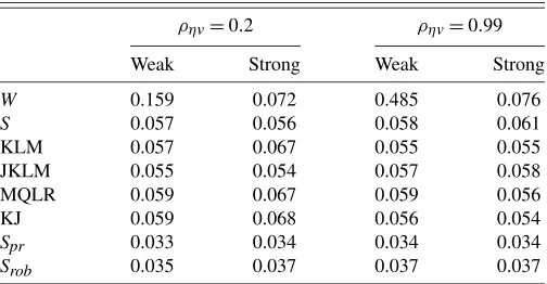
We compute the size and power of testing H0:γf =1/2
againstH1:γf =1/2 at the 5% significance level using a
two-step Wald statistic and the subsetS, KLM, JKLM, and MQLR statistics. The latter statistics all use the CUE for λ. Table 1 reports the rejection frequencies under the null hypothesis and Figures2and3show the resulting power curves of 5% signif-icance level tests of the null hypothesis H0:γf =1/2 against H1:γf =γf,1for values ofγf,1between zero and one. The left-hand sides correspond to weak instruments (the smallest eigen-value of the concentration matrix divided by the number of
in-Table 1. Null rejection frequencies of 5% level tests of the hypothesis
γf=0.5 against a two-sided alternative in the NKPC
ρηv=0.2 ρηv=0.99
Weak Strong Weak Strong
W 0.159 0.072 0.485 0.076
S 0.057 0.056 0.058 0.061
KLM 0.057 0.067 0.055 0.055
JKLM 0.055 0.054 0.057 0.058
MQLR 0.059 0.067 0.059 0.056
KJ 0.059 0.068 0.056 0.054
Spr 0.033 0.034 0.034 0.034
Srob 0.035 0.037 0.037 0.037
NOTE: The model isE[Zt(πt−λxt−γfπt+1] =0, whereZtincludes the first three lags
ofπt,xt.Newey and West (1987)weight matrix. The smallest eigenvalue of the
concen-tration matrix per instrument(μ2/k)is 1 for weak and 30 for strong identification. 10,000 Monte Carlo replications.
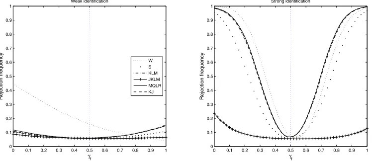
Figure 2. Power curves of 5% level tests forH0:γf =0.5 againstH1:γf =0.5. The sample size is 1,000 and the number of MC replications
is 10,000.
struments,μ2/k, is equal to 1), while the right-hand sides cor-respond to strong instruments (μ2/k=30). The power curves reported in the figures are for the caseρηv=0.2, for which the
associated null rejection frequencies are given in the left two columns of Table1.
Table1also reports the rejection frequencies of the tests with identical values ofμ2/kbut with a different value of the correla-tion coefficient of the errors,ρηv=0.99. The results show that
the Wald statistic is size distorted in the case of weak instru-ments, while the size of all other statistics is around or below 5%. Table1 also shows that the projection and Robins-based
S-tests are conservative.
Figure2shows that under weak instruments the Wald statis-tic is severely size distorted while the power of all identification robust tests is similar and small. Under strong instruments, the power curves that result from the KLM and MQLR statistics are indistinguishable and theS-test is less powerful. The size of the Wald test is improved relative to the weak instruments case, but it is still higher than the nominal level.
Figure 3 compares the power of the subsetS-test with the projection-based versionSpras well as the Robins version,Srob
the latter relying on a 2% level KLM pretest forλ. The subset
S-test dominates both of the other two versions.
In the linear instrumental variables regression model with homoscedastic errors and one included endogenous variable the MQLR statistic coincides with the CLR statistic of Mor-eira (2003). In that model,Andrews, Moreira, and Stock (2006) show that the MQLR statistic is the most powerful statistic for testing two-sided hypotheses. They obtain this result by con-structing the power envelope, which results from point optimal test statistics, and showing that the power curve that results from the MQLR statistic coincides with the power envelope. Figure2shows that the MQLR statistic is the preferred statistic for testing hypotheses on subsets of the parameters in GMM in our simulation experiment as well. An extension of this result to the general case of testing hypotheses on subsets of the pa-rameters in GMM has not been established. We consider it an important topic for further research.
5. ESTIMATION RESULTS
We estimate the NKPC model using quarterly data for the U.S. economy over the period 1960 quarter 1 to 2007 quar-ter 4. Inflation is measured by 100 times ln(Pt), where Pt
is the gross domestic product (GDP) deflator, obtained from the
Figure 3. Comparison of the power curves of 5% level subset, projection and Robins (2004)S-tests forH0:γf =0.5 againstH1:γf =0.5.
The sample size is 1,000 and the number of MC replications is 10,000.
FRED database of the St. Louis Fed. FollowingGalí and Gertler (1999), we use the labor share as a proxy for marginal costs. Use of alternative measures, such as the estimate of the output gap provided by the Congressional Budget Office (CBO), de-trended output, or output growth, produce similar results (point estimates ofλare different, notably negative when output gap is used, but the confidence intervals are very similar in all cases). The data for the labor share were obtained from the Bureau of Labor Statistics (BLS, series ID: PRS85006173). To ensure our estimates of the slope coefficientλare comparable to those reported inGalí and Gertler (1999), we scale the log of the la-bor share by a constant factor of 0.123, as they do. This factor depends on two unidentifiable structural parameters, and only affects the interpretation of the coefficientλ.
We estimate the NKPC model (2) by the CUE, using three lags of inflation and the labor share as instruments and the Newey and West (1987)heteroscedasticity and autocorrelation consistent (HAC) estimator of the optimal weight matrix. The point estimates and the bounds of 95% confidence sets de-rived by inverting the subset MQLR statistic are reported in the first column of Table2. We also report the result of the Hansen (1982)test of overidentifying restrictions, which is cor-rectly sized when evaluated at the CUE, as explained above. Thep-value for the Hansen test is about 0.5, showing no ev-idence against the validity of the moment restrictions at con-ventional significance levels. These results are not sensitive to the choice of HAC estimator. For example, they are almost the same if we use the quadratic spectral kernel estimator proposed byAndrews and Monahan (1992)or the MA-l estimator pro-posed byWest (1997).
The point estimates we obtain are comparable to those found in many other studies that use a similar limited information approach. The slope of the Phillips curve is estimated to be positive but small, and notably insignificantly different from zero. The forward-looking coefficientγf is about 3/4 and
dom-inates the backward-looking coefficient, which is about 1/4. However, the confidence intervals are relatively wide, and no-tably wider than the Wald-based confidence intervals reported in most other studies. Thus, we cannot reject at the 5% level the
Table 2. Estimates of the NKPC
Parameter Unrestricted Restricted (γf+γb=1)
λ 0.035 0.039
[−0.053, 0.170] [−0.049, 0.167]
γf 0.773 0.770
[0.531, 1.091] [0.556, 1.053]
γb 0.230
[−0.062, 0.451]
γf+γb−1 0.003
[−0.046, 0.059]
Hansen test 2.486 2.492
p-value 0.478 0.477
NOTE: The model isE[Zt(πt−c−λxt−γfπt+1−γbπt−1)] =0. Instruments include
a constant and three lags ofπt,xt(lags ofπtare replaced by lags ofπtin the restricted
model). Point estimates are derived using CUE-GMM withNewey and West (1987)weight matrix; square brackets contain 95% confidence intervals based on the subset MQLR test. The estimation sample is 1960 quarter 1 to 2007 quarter 3.
pure NKPC model that arises whenγb=0. This seems counter
to the conventional view (see, e.g., Galí and Gertler1999) that some degree of “intrinsic” persistence is necessary to match the observed inflation dynamics. We shall investigate later the ro-bustness of these results to changes in the instruments and esti-mation period.
Many studies of the hybrid NKPC impose the restriction that the forward and backward coefficients sum to one, that is, γf +γb=1;see Buiter and Jewitt (1989),Fuhrer and Moore
(1995),Christiano, Eichenbaum, and Evans (2005), andRudd and Whelan (2006). Even though formal theoretical justifica-tion for this restricjustifica-tion can be provided from microfoundajustifica-tions (see, e.g., Galí and Gertler 1999; Woodford2003, chapter 2; and Christiano, Eichenbaum, and Evans2005), the motivation for it has largely been empirical. Indeed, our estimates reported in Table 2 indicate that γf +γb is not significantly different
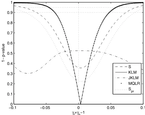
from one, in line with most other studies. To shed further light on this, we report 1−p-value plots for various identification ro-bust (subset) tests on the parameterδ=γf+γb−1 in Figure4.
The null hypothesisγf +γb=1 is not rejected at conventional
significance levels by any of the tests. It is also noteworthy that the parameter γf +γb−1 is very accurately estimated, since
the 95% level MQLR confidence interval reported in Table2is very tight around zero.
It may be thought that imposing the restrictionγf +γb=1
will improve the identifiability of the structural parameters λ, γf. This argument was made, for example, in Jondeau and
Le Bihan (2008). To investigate this possibility, we reestimate the NKPC under the restrictionγf +γb=1, and the results are
reported in the second column of Table2. It is clear that the fit of the model, as indicated by Hansen’s (1982) overidentification statistic, is essentially not altered. Moreover, by comparing the confidence intervals forλandγf reported in the two columns
of Table 2, we notice that they shrink very little when the re-striction is imposed. Intuitively, imposing rere-strictions can help identification mainly when the restrictions are placed in direc-tions of the parameter space where identification is weak. The
Figure 4. Identification robust tests of the hypothesisγf+γb=1.
The figure reports 1−p-value plots for different values of coefficient
γf+γb−1.
restrictionγf +γb=1 does not improve the identifiability ofλ
andγf because the parameterγf+γbis rather well identified.
In fact, all of our subsequent results are essentially unaffected by whether we impose the restriction γf +γb=1 or not, so,
for simplicity, we shall report only the results of the restricted model. There is one other complication that we need to account for when we estimate the restricted model, which relates to the persistence in the observed data. When γf ≤1/2, the unique
stable solution forπt in the restricted model is (see Rudd and
Whelan2006):
πt= λ 1−γf
∞
j=0
γ
f
1−γf
j
Et(xt+j)+ut.
When the labor share,xt, is stationary and not Granger-caused
byπt, as Equation (4) above, it follows thatπthas a unit root.
Thus, using lags of πt as instruments would violate the
con-ditions for the asymptotic theory given in Section 3. In other words, the identification robust tests need not control size when the instruments are nonstationary. To avoid this problem, we use lags ofπt(instead of lags ofπt) as instruments. This is also
done inRudd and Whelan (2006). See alsoMavroeidis (2006) for further details on this issue. We should point out, for com-pleteness, that the restricted model does not necessarily imply that inflation has a unit root. Whenxt is Granger-caused byπt,
the dynamics ofπt are determined by a vector autoregression
in(πt,xt), and stationarity depends on the roots of the
charac-teristic polynomial. Moreover, even in the case whenxt is not
Granger-caused byπt, whenγf >1/2, the solution of the model
is of the form (see Rudd and Whelan2006):
πt=
1−γf
γf
πt−1+
λ γf
∞
j=0
Et(xt+j)+ut,
which is stationary wheneverxt is stationary. However, use of
lags ofπtas instruments is robust across all values ofγf and
independent of whetherxt is Granger-caused by πt, so this is
what we do hereafter. It is interesting to note that the empirical results do not depend much on whether lags ofπt orπt are
used in the instrument set. The confidence sets we report would be slightly wider if we used πt−1, πt−2, and πt−3 instead of πt−1, andπt−2as instruments. None of our conclusions is affected by this choice of instruments.
5.1 One-Dimensional Confidence Sets
Under the restrictionγf +γb=1, model (2) can be rewritten
as
πt=λxt+γf(πt+1−πt−1)+et. (32)
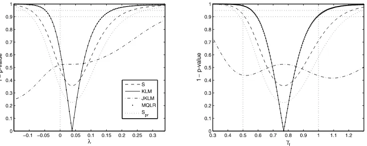
Figure5 reports 1−p-value plots associated with the subset tests on each of the parametersλandγf. The 95% MQLR
con-fidence bounds reported in the second column of Table2 coin-cide with the intersections of the 1−p-value plot for the MQLR statistic with the 0.95 line. We observe that the MQLR plot is almost indistinguishable from the KLM plot, leading to identi-cal confidence sets. The confidence sets derived from theS-test are wider, but shorter than the projection-basedSpr-test, as
ex-pected. The JKLM test indicates no violation of the moment conditions for any value of the parameters that are within the MQLR and KLM 90% and 95% level confidence sets.
The following conclusions can be drawn from the above re-sults. First, even though the slope of the Phillips curve is esti-mated to be positive, it is not significantly different from zero at the 35% level according to any of the tests. This conclusion is consistent with the findings ofRudd and Whelan (2006), and it is robust to using additional instruments, as inGalí and Gertler (1999)andRudd and Whelan (2006). One interpretation is that the labor share is not a relevant determinant of inflation. This in-terpretation is not uncontroversial.Kuester, Mueller, and Stoelt-ing (2009)argue that the baseline NKPC yields downwardly biased estimates ofλ (the sensitivity of inflation to marginal costs) due to the omission of persistent cost-push shocks. The result remains unchanged when we replace the labor share with other measures of marginal costs, such as the output gap or real output growth.
Second, the coefficientγf is not very accurately estimable.
This is not surprising, given our earlier discussion about the effects of a small value of λon the identifiability of γf. It is
important to note, however, thatγf is not completely
uniden-tified. Specifically, most of the 95% level confidence sets ex-clude values ofγf close to zero. According toGalí and Gertler
(1999), this can be interpreted as evidence of forward-looking behavior in price setting, though this interpretation is not un-controversial (cf. Mavroeidis2005or Rudd and Whelan2005). The smallest 95% level confidence interval ofγf is obtained
by inverting the MQLR test, and it includes the valueγf =1,
Figure 5. 1−p-value plots for the coefficiens(λ, γf)in the NKPC model, under the restrictionγf+γb=1.