Full Terms & Conditions of access and use can be found at
http://www.tandfonline.com/action/journalInformation?journalCode=ubes20
Download by: [Universitas Maritim Raja Ali Haji] Date: 11 January 2016, At: 22:58
Journal of Business & Economic Statistics
ISSN: 0735-0015 (Print) 1537-2707 (Online) Journal homepage: http://www.tandfonline.com/loi/ubes20
Dynamic Factor Models for Multivariate Count
Data: An Application to Stock-Market Trading
Activity
Robert C. Jung, Roman Liesenfeld & Jean-François Richard
To cite this article: Robert C. Jung, Roman Liesenfeld & Jean-François Richard (2011) Dynamic Factor Models for Multivariate Count Data: An Application to Stock-Market Trading Activity, Journal of Business & Economic Statistics, 29:1, 73-85, DOI: 10.1198/jbes.2009.08212
To link to this article: http://dx.doi.org/10.1198/jbes.2009.08212
Published online: 01 Jan 2012.
Submit your article to this journal
Article views: 287
View related articles
Dynamic Factor Models for Multivariate Count
Data: An Application to Stock-Market
Trading Activity
Robert C. JUNG
Department of Economics, Universität Erfurt, 99089 Erfurt, Germany (robert.jung@uni-erfurt.de)
Roman LIESENFELD
Department of Economics, Christian-Albrechts-Universität zu Kiel, 24118 Kiel, Germany (liesenfeld@stat-econ.uni-kiel.de)
Jean-François RICHARD
Department of Economics, University of Pittsburgh, Pittsburgh, PA 15260 (fantin@pitt.edu)
We propose a dynamic factor model for the analysis of multivariate time series count data. Our model allows for idiosyncratic as well as common serially correlated latent factors in order to account for po-tentially complex dynamic interdependence between series of counts. The model is estimated under al-ternative count distributions (Poisson and negative binomial). Maximum likelihood estimation requires high-dimensional numerical integration in order to marginalize the joint distribution with respect to the unobserved dynamic factors. We rely upon the Monte Carlo integration procedure known as efficient im-portance sampling, which produces fast and numerically accurate estimates of the likelihood function. The model is applied to time series data consisting of numbers of trades in 5-min intervals for five New York Stock Exchange (NYSE) stocks from two industrial sectors. The estimated model provides a good parsimonious representation of the contemporaneous correlation across the individual stocks and their serial correlation. It also provides strong evidence of a common factor, which we interpret as reflecting market-wide news.
KEY WORDS: Dynamic latent variables; Importance sampling; Mixture of distribution models; Pois-son distribution; Simulated Maximum Likelihood.
1. INTRODUCTION
Modeling dispersion and serial correlation for univariate count series received much attention over recent years. Exist-ing approaches can be broadly classified as either observation or parameter driven. The monographs of Kedem and Fokianos (2002) and McKenzie (2003) provided excellent overviews.
Multivariate dynamic models for count data remain few. As discussed by Cameron and Trivedi (1998, section 8.1), this might be explained by the fact that classical inference in multi-variate count data models has proven to be analytically as well as computationally demanding. Pioneering multivariate appli-cations are found in Jørgensen et al. (1999), Held, Hohle, and Hofmann (2005), Heinen and Rengifo (2007), and Quoreshi (2008). The specification proposed by Jørgensen et al. (1999) belongs to the class of parameter-driven models. It consists of a multivariate Poisson state–space model with a common factor that can be analyzed by a Kalman filter. It is used to assess the impact of air pollution on daily emergency admission counts in a hospital for four sickness categories. Held, Hohle, and Hof-mann (2005) and Quoreshi (2008) proposed observation-driven models that are based upon a vector autoregressive moving av-erage (VARMA) structure. The model of Held, Hohle, and Hof-mann imposed a simple vector autoregressive (VAR) structure for the conditional means and is applied to infectious disease surveillance counts from a measle epidemic. The specification of Quoreshi represented a multivariate extension of the univari-ate integer-valued autoregressive moving average (INARMA)
models introduced by McKenzie (1986) and Al-Osh and Alzaid (1987) and is used to study spillover effects in the stock trading activities of two individual stocks. Both models are amenable to standard methods of estimation, but are parameter rich. In order to analyze comovements in the number of trades for five individual stocks, Heinen and Rengifo (2007) also adopted an observation-driven approach extending the univariate autore-gressive conditional Poisson model of Heinen (2003). A cop-ula approach is used to represent contemporaneous correla-tions among time series counts. Since efficient joint maximum-likelihood (ML) estimation is not feasible, the authors rely upon a consistent, though less efficient, two-stage ML approach for separate estimation of the parameters of the marginal distribu-tions and of those of the copula. Other multivariate count mod-els rely upon panel data techniques, with an emphasis on unob-served heterogeneity in the individual series. See Winkelmann (2008) for a recent survey.
In the present article we adopt a parameter-driven approach and propose a new flexible, parsimonious, and easy-to-interpret dynamic factor model for multivariate count series. It builds upon and generalizes earlier models by Jørgensen et al. (1999) and Wedel, Bockenholt, and Wagner (2003). The former model includes only a single dynamic common factor and no dynamic
© 2011American Statistical Association Journal of Business & Economic Statistics January 2011, Vol. 29, No. 1 DOI:10.1198/jbes.2009.08212
73
idiosyncratic components. The latter model is a static multi-variate Poisson factor model for cross-sectional analyses. Our model allows for serially correlated common as well as idiosyn-cratic factors driving the conditional means of the count distri-butions. Therefore, it can account for nontrivial contemporane-ous as well as temporal interactions across count series. It can also accommodate different distributional assumptions for the conditional distribution of the counts given the factors. This can be critical since the commonly used Poisson distribution has an index of dispersion equal to 1 (the latter being defined as the ratio between the variance and the mean). However, count data often exhibit strong over-dispersion (index significantly larger than 1), which cannot be fully captured by a conditional Pois-son distribution even if marginalization of the conditional mean can generate by itself an over-dispersed unconditional distribu-tion. Hence, it might be important to allow for conditional dis-tributions that can accommodate over-dispersion, such as the negative binomial (hereafter Negbin).
The dynamic latent factors enter our model nonlinearly. Thus, likelihood evaluation requires high-dimensional numer-ical integration, for which we use the efficient importance sampling (EIS) procedure developed by Richard and Zhang (2007). EIS is a generic, flexible, and easy-to-implement Monte Carlo (MC) integration procedure specifically designed to max-imize numerical accuracy. It also facilitates exploring alterna-tive model specifications that typically require only minor mod-ifications of a baseline EIS implementation. Last but not least, EIS can be used to compute filtered estimates of the latent fac-tors themselves. Several diagnostic test statistics are based upon such estimates.
We apply our model to a multivariate time series consisting of numbers of trades in 5-min intervals for five stocks traded at the New York Stock Exchange (NYSE). We implicitly adopt the information flow interpretation associated with the mixture-of-distribution model of Tauchen and Pitts (1983). See also An-dersen (1996) and Liesenfeld (2001). In this context, numbers of trades are directly influenced by the arrival of new informa-tion, whether specific to a single stock (idiosyncratic factor), to an industry (sector factor), or to the market (market factor). Be-cause news arrivals also drive the volatility of asset returns, our specification for the number of trades is intimately related to the dynamic latent factor models for the volatility of multivariate return series proposed by Diebold and Nerlove (1989), Aguilar and West (2000), and Chib, Nardari, and Shephard (2006).
Alternative multivariate approaches used to analyze the stock market trading activity are based on the duration between suc-cessive trades or the trading intensity defined as the instan-taneous rate of trade occurrence. Spierdijk, Nijman, and van-Soest (2002), for example, proposed a bivariate duration model for two stocks, which combines a univariate model for the “pooled” durations between two successive trades in any of the two stocks with a Probit model that determines which of the two stocks is traded. However, the application of this model to more than two stocks becomes intractable. A multivariate ap-proach based on the intensity that is applicable to a larger num-ber of stocks and which is closely related to ours is proposed by Bauwens and Hautsch (2006). They considered a model for price intensities that allows for observation-driven stock-specific intensity components and for a latent dynamic common
component that jointly drives the intensity of all stocks. Since their model is nonlinear in the dynamic latent common factor they also use EIS integration to obtain ML-estimates.
The article is organized as follows. The multivariate dynamic factor model is introduced in Section 2. Section 3 discusses ML estimation and filtering based upon EIS. The application to NYSE data is presented in Section4. Section5concludes.
2. DYNAMIC FACTOR MODEL FOR MULTIVARIATE COUNT DATA
The econometric model we propose consists of a dynamic extension of the static multivariate Poisson factor model intro-duced by Wedel, Bockenholt, and Wagner (2003). Consider a
J-dimensional vector of countsyt=(yt1, . . . ,ytJ)′recorded at timet(t=1, . . . ,T). Dynamics will be introduced at the level of the latent factors. Accordingly, counts are assumed to be con-ditionally independently distributed with Poisson distributions
p(ytj|θtj)=
whose meansθtj are latent random variables. We assume the existence of a link function b(·), whereby the mean vector
θt=(θt1, . . . , θtJ)′ can be expressed as a linear function of a
P-dimensional vector of latent random factorsft, say
b(θt)=μ+Ŵft, (2) whereμdenotes a vector of fixed intercepts andŴa(J×P) ma-trix of factor loadings. ThePlatent factors inftare assumed to be independent of each other. A log-link functionb(θt)=ln(θt) is convenient since it implies positivity ofθtwithout parametric restrictions on(μ,Ŵ)and is the only one considered here.
In the context of our NYSE application considering the joint behavior of the number of trades for different stocks, we allow for a single common market factorλt,S<J industry-specific factorsτt =(τt1, . . . , τtS)′, and J stock-specific factors ωt = (ωt1, . . . , ωtJ)′. Hence, ft is partitioned into ft =(λt,τ′t,ω′t)′ andP=J+S+1. The matrix of factor loadings is partitioned conformably withft intoŴ=(Ŵλ,Ŵτ,Ŵω), whereŴλ=(γjλ)
is aJ-dimensional vector,Ŵτ=(γjτs)aJ×Smatrix with zero entries for any firm j that does not belong to sector s, and
Ŵω=diag(γ ωj
j )a(J×J)diagonal matrix. Thus, the log-mean function for stockj, belonging to industrysis given by
lnθtj=μj+γjλλt+γ
τsj
j τtsj+γ
ωj
j ωtj, (3)
where the indexsjdenotes the industry of firmj.
In order to account for possible serial and cross-correlation in the counts, we assume that the factors follow independent Gaussian AR(1)processes, say
λt|λt−1∼N(κλ+δλλt−1,[νλ]2), (4)
τts|τt−1s∼N(κτs+δτsτt−1s,[ντs]2), (5)
ωtj|ωt−1j∼N(κωj+δωjωt−1j,[νωj]2). (6)
To ensure stationarity of the factors, it is assumed that|δλ|<1,
|δτs|<1, and|δωj|<1. Other distributional and dynamic spec-ifications for the factors are easily accommodated. Under an
identity linkb(·), for example, Gamma or log-normal transition distributions will provide suitable factor specifications (see Jør-gensen et al.1999and Jung and Liesenfeld2001). Also, higher order AR(p) processes can be accommodated.
The model as specified is unidentified. Identification for the static case with iid factors is discussed in Wedel, Bockenholt, and Wagner (2003) and can be extended to the dynamic model introduced here. We impose the restrictions that κλ =κτs = κωj =0 for s=1, . . . ,S and j=1, . . . ,J in order to identify theμj’s [see Equations (4)–(6)]. Furthermore, we setγjωj=1 forj=1, . . . ,J,γτs
j =1 for one arbitrarily selected stock jin industrysfor s=1, . . . ,S, andγjλ=1 for one arbitrarily se-lected stockj[see Equation (3)]. This eliminates indetermina-cies in the factor scales.
Under the assumed Poisson distribution, whose dispersion index equals 1, over-dispersion of the counts can only orig-inate from the unconditional variances of the factors, which themselves critically depend on the persistence parameters (δλ, δτs, δωj). In order to relax this close relationship between over-dispersion and persistence, we will substitute the more flexible Negbin distribution for the Poisson. It is given by
p(ytj|θtj)=
whereŴ(·) denotes the Gamma function. Its mean and vari-ance are given byθtj andθtj(1+σj2θtj), respectively. Its over-dispersion is a monotone increasing function ofσj>0 and the Poisson distribution in Equation (1) obtains as the limit for σj→0.
3. EIS BASED INFERENCE
In order to estimate the model we use ML based upon EIS. An alternative will be to use GMM based on unconditional mo-ments that can be computed in closed form. However, it is well known that for models with dynamic latent factors a likelihood-based approach has typically better finite-samples properties than GMM—see, e.g., Andersen, Chung, and Sørensen (1999).
3.1 EIS
The evaluation of the likelihood function for the model de-scribed by Equations (1) to (6) requires integrating the joint density of counts and factors with respect to the T·P latent factor variables (in our applicationT·Pequals 36,600). For the likelihood evaluation, counts are kept fixed at their observed values and are, therefore, omitted from notation except for the fact that densities need to be time indexed to reflect their depen-dence on the data. The likelihood integral to be evaluated is of the form: whereψ regroups the parameters of the model andϕt denotes the product of the timetdensities forytgivenftand forftgiven
ft−1 as defined by Equations (1) to (6). The initial condition
f0 is assumed to be the known constantf0=E(ft)=0. Since
ft is serially dependent and enters the model nonlinearly the likelihood integral in Equation (8) is not amenable to standard integration procedures.
Following Richard and Zhang (2007), the EIS MC integra-tion for the likelihood in Equaintegra-tion (8) is based upon a sequence of auxiliary importance sampling densities forft givenft−1of the form (preselected) class of auxiliary parametric density kernels with known analytical integrating factors in ft given ft−1 denoted byχt(ft−1;at). The likelihood integral in Equation (8) is then portance sampling MC estimate of the likelihoodL(ψ)is given by from the sequence of importance sampling densities {mt(ft |
ft−1;at)}Tt=1. EIS aims at selecting values of the auxiliary pa-rameters {at}that minimize the MC sampling variance of the MC estimate in Equation (11). This requires minimizing period by period the variance of the ratiosϕt·χt+1/kt as functions of
ft and ft−1 with respect to the mt-distributions. As shown in Richard and Zhang (2007), an MC-EIS approximate solution of this minimization problem obtains from the following back-ward recursive sequence of auxiliary least squares (LS) prob-lems:
t=1 denotes a trajectory drawn from an initial se-quence of auxiliary samplers {mt(ft |ft−1;a(t0))}Tt=1 with i= 1, . . . ,N (iid). As initial samplers we use the Gaussian densi-ties associated with second-order Taylor-series approximations (TSA) to ϕtχt+1 as described below. As detailed in Richard and Zhang (2007), the sequence of EIS auxiliary regressions in Equation (12) is iterated by replacing the initial auxiliary
samplers by the previous stage importance samplers. For such iterations to converge to a fixed-point solution for{ˆat}, char-acterizing the final EIS sampling densities{mt(ft|ft−1; ˆat)}, it is critical that allith trajectories{˜f(ti)}T
t=1be obtained by trans-forming a single set of common random numbers (CRNs), say
{ ˜u(ti)}T
t=1. CRNs are N(0,1)for Gaussian EIS samplers. The MC-EIS evaluation of L(ψ) for a given value of ψ
then obtains by substituting the fixed-point values of {ˆat}for
{at}in Equation (11). A generalization of Equations (4)–(6) to higher order AR(p) processes only requires replacing in Equa-tions (8)–(12)ft−1byFt−1=(ft′−1, . . . ,f′t−p)′andf0byF0(see Richard and Zhang2007).
Note that{ˆat}is an implicit function ofψ. Therefore, max-imal numerical efficiency requires complete reruns of the EIS algorithm for any new value ofψ. The (re)use of CRNs across those reruns ensures continuity of the MC likelihood evaluation
¯
LN(ψ)with respect toψ, which is critical for likelihood maxi-mization. Finally, it should be mentioned that EIS-density ker-nelskt within the exponential family of distributions are linear in the auxiliary parametersatunder their natural parameteriza-tion as well as closed under multiplicaparameteriza-tion. As detailed below, these two properties considerably simplify the application of EIS to our model.
3.2 Implementation of EIS for the Poisson Factor Model
The implementation of the sequential EIS procedure outlined in Section 3.1 for the model defined by Equations (1) to (6) proceeds as follows. Under the log-link function, the Poisson density in Equation (1) is rewritten as
p(ytj|φtj)= density of the conditional Gaussian distribution forftgivenft−1 has the form
whereandHare both diagonal andHdenotes the inverse of the covariance matrix offtgivenft−1.
In order to apply sequential EIS to this model, we first note that the factorϕt(ft,ft−1;ψ)in the likelihood integral in
Equa-whereφtjis a linear function inft. Next, note that if the selected kernelkt(ft,ft−1;at)in Equation (9) is Gaussian in bothftand
ft−1, then its integrating constantχt(ft−1;at)is itself Gaussian in ft−1. By recursion this implies that the sole non-Gaussian
term in the product ϕtχt+1 to be approximated by kt via the EIS auxiliary regressions in Equation (12) is the product of the
J densities p(ytj|φtj). Thus, it suffices to construct Gaussian approximates in φtj to the latter densities in order to produce a Gaussian kernelktfor(ft,ft−1). The corresponding kernelkt consists of the product:
kt(ft,ft−1;at)=p(ft|ft−1;ψ)ζt(ft;at)χt+1(ft;at+1), (17)
whereζtdenotes the product ofJunivariate Gaussian kernels in φtjdesigned to approximateJj=1p(ytj|φtj). It is parameterized
whereBt=diag(btj)denotes aJ×Jpositive-definite diagonal matrix and ct=(ctj) a J-dimensional vector. The EIS auxil-iary parameterat is defined asa′t=(vech(Bt)′,c′t). Note that the factors lnp(ft|ft−1;ψ)and lnχt+1appear on both sides of the auxiliary EIS regression in Equation (12) and cancel out. It follows that this regression simplifies intoJindependent linear LS regressions of{lnp(ytj| ˜φtj(i))}Ni=1on{(φ˜tj(i),[ ˜φtj(i)]2)}Ni=1with intercepts.
Since the density kernels kt in Equation (17) depend on the one-period ahead integrating constantsχt+1, they are ob-tained back-recursively as described next. Sinceχt+1is itself a Gaussian kernel inft, we introduce the following auxiliary parameterization:
EIS auxiliary parameterat+1 resulting from the backward re-cursion as given below. SinceχT+1≡1, the “initial values” are
PT+1=0,qT+1=0, andrT+1=0. Next, we combine together
It immediately follows from Equation (20) that the Gaussian EIS sampler forft|ft−1is given by
mt(ft|ft−1;at)∼N(dt+Gtft−1,M−t 1). (22)
The integrating constantχt(ft−1;at)obtains by regrouping all remaining factors in Equation (20) and is, therefore, of the form introduced in Equation (19) together with
Pt=′H−G′tMtGt,
qt=G′tMtdt,
(23)
rt=μ′Btμ−2μ′ct+rt+1−d′tMtdt
+ln|H−1| −ln|M−t 1|.
In summary, the computation of the EIS estimate of the likeli-hood requires the following simple steps:
Step(i). Generate N independent P-dimensional trajecto-ries{{˜f(ti)}T Equations (21)–(23) in order to construct the initial EIS sam-plers.
Step(ii). Transform the simulated ft-trajectories from the previous sampler into the corresponding N independent J -dimensionalφt-trajectories according toφt=μ+Ŵft. The lat-ter are used to solve back recursively the LS-problems in Equa-tion (12). This requires running the following J independent linear auxiliary regressions for each periodt:
lnpyt1| ˜φt(1i)=constant−
Step(iii). Use the LS estimates of the auxiliary parameters
ˆ
Bt=diag(bˆtj)andcˆt=(cˆtj)obtained in step (ii), to construct back-recursively the sequence of EIS-sampling densities{m(ft|
ft−1,aˆt)}as given by Equation (22) together with the recursions in Equations (21) and (23).
Step(iv). Generate N independent trajectories from the se-quence of EIS samplers constructed in step (iii) and use them either to repeat steps (ii) and (iii) or (at convergence) to com-pute the EIS-MC estimate of the likelihood according to Equa-tion (11).
If we replace the Poisson density in Equation (1) by the Negbin density in Equation (7), we only need to modify ac-cordingly the dependent variables in the auxiliary EIS regres-sions, a trivial adjustment altogether. For a generalization of Equations (4)–(6) to higher order AR(p) processes we need to modify accordingly the transition density in Equation (15) and to adjustχt+1in Equation (19) to be a Gaussian kernel in
Ft=(f′t, . . . ,f′t−p+1)′.
3.3 Filtering and Diagnostics
In state–space applications such as the one analyzed here, in-terest lies also in the filtered values of the latent states (factors) whether for diagnostic checking or forecasting. Filtering entails the computation of the conditional expectation of some function
h(ft)(includingft itself) given the information available up to timet−1 denoted byYt−1. This expectation takes the form of (15) and (16), respectively. These integrals are functionally sim-ilar to the likelihood integral in Equation (8) and can, in turn, be accurately approximated by EIS (see Liesenfeld and Richard
2003).
Filtering enables us to compute the standardized Pearson residuals defined as
ztj= [ytj−E(ytj|Yt−1)]/Var(ytj|Yt−1)1/2. (27)
These residuals are critical components of a variety of diagnos-tic statisdiagnos-tics since they should have zero mean, unit variance, and be serially uncorrelated if the model is correctly specified. Under the Poisson model, the relevant conditional moments of
ytj are given by E(ytj|Yt−1)=exp{μj} ·E(exp{γ′jft} |Yt−1)
and Var(ytj|Yt−1)=exp{μj} ·E(exp{γ′jft} |Yt−1)+exp{2μj} · Var(exp{γ′jft} |Yt−1), whereγ′jdenotes thejth row of the load-ing matrixŴ.
In order to check the distributional assumptions of the fac-tor model we use the “randomized” version of the probabil-ity integral transform (PIT) proposed by Liesenfeld, Nolte, and Pohlmeier (2006). The PIT values of a random variable consist of its predictive cdf evaluated at the observed values. If the pre-dictive cdf is correctly specified and continuous, the PIT values follow a standard uniform distribution (see Rosenblatt1958). The randomized PIT approach accounts for the fact that the PIT values for discrete predictive cdf’s are no longer uniform. Let{yotj}denote the actual count observations. The application of randomized PIT to theJcount series is based on simulated random drawsu˜tj(t=1, . . . ,T;j=1, . . . ,J) from uniform
dis-If the model is correctly specified,u˜tjis a serially independent random variable following a uniform distribution on the inter-val[0,1]. Using the inverse of a standardized Gaussian cdf, the
variableu˜tjcan be mapped into a N(0,1)-distribution:
z∗tj=−1(u˜tj), (29) such that the resulting normalized PIT residualsz∗tj should fol-low a standard normal distribution. The probability c(tju) in Equation (28) obtains by setting the function h(ft) in Equa-probabilityc(tjl)obtains analogously.
4. APPLICATION TO STOCK–MARKET ACTIVITY
The dynamic factor model for counts introduced in Section2
is used to analyze the dynamics and correlations of stock mar-ket activity measured by the number of trades aggregated over time intervals with a fixed length. Note that time aggregation of the irregularly spaced trading events entails a loss of informa-tion on the dynamics of the trading process, which is increas-ing with the interval size. This raises the question of the “opti-mal” length of the aggregation interval. Following Heinen and Rengifo (2007) and Quoreshi (2008), we use an interval length of 5 min—a choice that is regarded as a good compromise be-tween keeping the information loss low and avoiding too many zeros for intervals which are too small.
4.1 The Data
The dynamic factor model is applied to the number of trades in 5-min intervals between 9:45 a.m. and 4:00 p.m. for J=5 stocks from two industry sectors traded at the NYSE: P.H. Glat-felter Company (GLT), Wausau Paper Corporation (WPP), Em-pire District Electric Company (EDE), Northeast Utilities (NU), and Westar Energy, Inc. (WR). The first two belong to the in-dustry subsector paper and the last three to the inin-dustry subsec-tor conventional electricity. Data are taken from the Trades and Quotes (TAQ) dataset, provided by the NYSE. The time period covered is the first quarter of 2005 (January 3, 2005–March 31, 2005) with 61 trading days. As there are 75 5-min intervals per day, the sample size isT=4575. See the top panel of Figure2
(in Section4.2.1) for time series plots of the number of trades. Descriptive statistics are provided in Table1and Table2reports the sample correlations across the five stocks, all of which are positive. The empirical distribution of the number of trades is clearly over-dispersed. The Ljung–Box statistics for the number
Table 1. Descriptive statistics for the number of trades
GLT WPP EDE NU WR
Mean 5.80 7.90 3.47 10.41 9.61
Median 5 7 3 9 9
Standard dev. 4.09 5.85 3.11 5.87 5.91
Minimum 0 0 0 0 0
Maximum 54 43 25 48 59
Q10 2086 4057 1575 3452 4150 Q20 2549 5026 1908 3927 5942
NOTE: The number of observations per stock isT=4575. The Ljung–Box statistics Q10andQ20include 10 and 20 lags.
Table 2. Sample correlation matrix for the number of trades
GLT WPP EDE NU WR
GLT 1
WPP 0.238 1
EDE 0.256 0.256 1
NU 0.206 0.174 0.283 1
WR 0.168 0.183 0.184 0.216 1
of tradesQ10andQ20including 10 and 20 lags, respectively, in-dicate strong serial correlation.
It is well known that intra-day trading activity has a distinc-tive U-shape pattern (see, e.g., Admati and Pfleiderer1988). In order to capture it, we introduce a Fourier series for the inter-cept in the log-mean function in Equation (3). Specifically,μj is replaced by a cyclical termμtjdefined as
μtj=μj+α′xt, (30) with α′=(α1, . . . , α4) and x′t =(cos(2πt/75),sin(2πt/75), cos(4πt/75),sin(4πt/75)). EIS trivially accommodates such extension. Note that specification in Equation (30) imposes a common diurnal pattern for all stocks, thereby preserving par-simony for the multivariate model. This restriction is justified by the finding that the individual patterns obtained from esti-mating univariate specifications (not presented here) are quite similar across the five stocks.
4.2 Estimation Results
4.2.1 Poisson Factor Model. For the Poisson factor model with a single common market factorλt, two sector-specific fac-torsτtsj and five idiosyncratic factorsωtjthe log-mean function for stockjis given by
lnθtj=μtj+γjλλt+γ
3 =1 for normalization. Joint ML-EIS estimates based upon N =50 trajectories are found in Table 3. ML-EIS estimation requires approxi-mately 100 Broyden–Fletcher–Goldfarb–Shanno (BFGS) iter-ations and takes of the order of 200 min on a Core 2 Duo In-tel 2.7 GHz processor using GAUSS on Windows XP. MC nu-merical standard deviations of the ML-EIS parameter estimates used as measures of numerical precision are obtained from 20 iid ML-EIS estimations conducted under different CRN seeds (see Richard and Zhang2007for details). They indicate that the parameter estimates are numerically very accurate. The fact that such high accuracy obtains with as little asN=50 trajectories indicates that the likelihood integrands in Equation (10) are very well-behaved functions of the 36,600 latent factor variables and are accurately approximated by the EIS-sampler (using 73,200 auxiliary parameters). In particular, theR2’s of the EIS auxiliary LS-problems in Equation (12) are typically larger than 0.99.
All parameter estimates are reasonable and apart fromα4 sig-nificant at the 1% significance level. The estimates of the fac-tor loadingsγjλ,γτ1
j , andγ
τ2
j suggest that the trading activity of all stocks load significantly on the common market factor
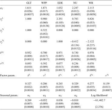
Table 3. ML-EIS for the dynamic Poisson factor model for the TAQ data
GLT WPP EDE NU WR
μj 1.611 1.871 1.032 2.247 2.113
(0.026) (0.017) (0.037) (0.012) (0.038) [0.0037] [0.0018] [0.0030] [0.0005] [0.0058]
γjλ 1.000 0.980 2.351 0.783 0.826
(0.060) (0.105) (0.040) (0.053) [0.0138] [0.0128] [0.0085] [0.0107]
γτ1
j 1.000 0.322 0.000 0.000 0.000
(0.052) [0.0181]
γτ2
j 0.000 0.000 1.000 −0.412 −2.122
(0.134) (0.237) [0.0132] [0.0116]
δωj 0.952 0.700 0.971 0.730 0.978
(0.009) (0.017) (0.007) (0.018) (0.004) [0.0011] [0.0017] [0.0009] [0.0026] [0.0005]
νωj 0.093 0.392 0.077 0.236 0.070
(0.010) (0.009) (0.013) (0.008) (0.008) [0.0011] [0.0012] [0.0017] [0.0012] [0.0009]
Factor param. δλ νλ δτ1 ντ1 δτ2 ντ2
0.327 0.206 0.245 0.329 0.277 0.139
(0.022) (0.007) (0.033) (0.009) (0.035) (0.013) [0.0018] [0.0011] [0.0033] [0.0022] [0.0034] [0.0007]
Seasonal param. α1 α2 α3 α4 Log-likelihood
0.269 −0.052 0.038 −0.010 −61,402.7 (0.007) (0.009) (0.009) (0.006)
[0.0008] [0.0010] [0.0005] [0.0005] [2.276]
NOTE: The reported numbers are the ML-EIS estimates for the parameters. Asymptotic standard errors obtained from a numerical approximation to the Hessian are in parentheses and MC (numerical) standard deviations obtained from 20 ML-EIS estimations conducted under different sets of CRNs are in brackets. ML-EIS estimates are based on a MC sample size ofN=50 and three EIS iterations.
λt and on their corresponding industry factor τt1 or τt2. The market factor appears to be dominated by EDE and the indus-try factors by GLT and WR, respectively. All factor loadings are positive except for the NU and WR loadings on the fac-tor of the electric-service industryτt2. Their negative signs, to-gether with the positive EDE loading onτt2, are indicative of a “substitution effect” in the trading activities of this sector. The estimates of the parameters for the market factor (δλ,νλ) and the two industry-specific factors (δτ1,ντ1,δτ2,ντ2) reveal that
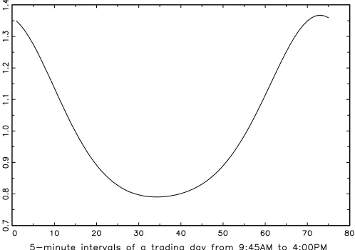
they exhibit substantial variation and a slight, yet significant, persistence. The estimates of the parameters characterizing the idiosyncratic factors (δωj,νωj) indicate substantially more per-sistence than for the common factors. Hence, the idiosyncratic factors appear to capture the persistent movements of the trad-ing process, while the common factors account for the more transitory variation. In light of the information-flow interpreta-tion associated with the mixture-of-distribuinterpreta-tion approach à la Tauchen and Pitts (1983), this suggests that market participants process market and industry-specific news significantly faster than firm-specific news. Figure1 shows the estimated diurnal seasonal effects for the number of trades. They exhibit the well-documented U-shape pattern.
The parameter estimates in Table3can be used to compute the implied estimates of the means and covariances of the un-conditional distribution for the number of trades, to be com-pared with their sample counterparts. In the presence of deter-ministic diurnal effects, the unconditional means and variances for the trades of stockjare given by
E(ytj)=ET(exp{μtj+0.5γ′jfγj}), (32) Var(ytj)=VarT(exp{μtj+0.5γ′jfγj})
+ET
exp{2μtj+γ′jfγj}[exp{γ′jfγj} −1]
+exp{μtj+0.5γ′jfγj}
, (33)
whereγjrepresents the vector of the factor loadings for stockj
andf the stationary covariance matrix of the vector of fac-tors ft. The notation ET and VarT indicate sample moments computed with respect to the deterministic variation of the di-urnal seasonal effects. The corresponding covariance between trading of stockj and stockkis obtained from the cross mo-ments
E(ytjytk)=ET
exp{μtj+μtk
+0.5(γj+γk)′f(γj+γk)}
, j =k. (34)
Figure 1. Estimated diurnal seasonal effects for the number of trades obtained under the Poisson factor model given by exp{0.269 cos(2πt/75)−0.052 sin(2πt/75)+0.038 cos(4πt/75)− 0.010 sin(4πt/75)}.
It can be shown that the resulting covariance Cov(ytj,ytk)is pos-itive (negative) as long asγ′jfγkis larger (smaller) than zero. The estimates of the unconditional mean and covariance matrix ofytare given by
respectively. The corresponding sample moments are
¯
respectively. The close match between those two sets of mo-ments indicates that the common factor model provides a good parsimonious representation of the contemporaneous correla-tion across the five stocks.
In order to assess the relative importance of the market factor, the industry factors, the idiosyncratic factors, and the diurnal component we computed their relative contribution to the over-all variance of the log-link function for the individual stocks lnθtj. The implied estimates of those contributions are reported in the upper panel of Table5 (in Section4.2.2). The fraction of variation explained by the market factor varies between 11%
(WPP) and 62% (EDE) while that of the industry-specific fac-tors range between 2% (NU) and 39% (GLT). Hence, the com-mon factors (market and industry), considered together, explain a significant fraction of the variation in the lnθtjs. However, these results also suggest that the industry factors might actu-ally capture additional firm-specific variations of GLT and WR rather than genuine industry-specific effects.
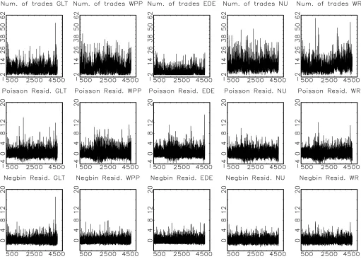
The upper panel of Table6(in Section4.2.2) summarizes the results of diagnostic checks on the Pearson residualsztjand the normalized PIT residualsz∗tj. Both sample means and standard deviations of the residualsztjexceed their respective benchmark values of 0 and 1 under a correctly specified model. This in-dicates that there is more variation and over-dispersion in the data than the model accounts for. This is confirmed by the in-spection of the time-series plots of theztj-residuals (see middle row of Figure2). The Jarque–Bera statisticJBgiven in Table6
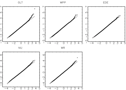
indicates a strong rejection of normality for thez∗tj’s suggesting that the model also has difficulties accounting for the skewness and tail behavior of the observed counts. This is corroborated by the quantile–quantile plots of thez∗tj’s provided in Figure3, which also confirm that the variance predicted by the model is too small to explain the variation in the data. Finally, the Ljung– Box statistics for the residuals ztj in Table6 indicate that the model does not fully capture the dynamic behavior of the trad-ing activity even though it dramatically reduces the correspond-ing statistics for the raw data as given in Table1.
4.2.2 Negbin Factor Model. In order to better account for over-dispersion and to allow for greater flexibility in capturing the serial correlation, we replace the conditional Poisson den-sity in Equation (1) by the Negbin density in Equation (7). As explained in Section3.2, this substitution only requires minor modifications of the baseline EIS algorithm.
The results of the ML-EIS estimation of the Negbin factor model are reported in Table4. The substitution of the Negbin for the Poisson distribution increases the value of the maxi-mized likelihood function by 193, indicative of a much better fit. Moreover, the additionalσ-parameters measuring the devi-ation from the Poisson distribution are all statistically signifi-cantly larger than zero. Nevertheless, the estimates of the in-tercept parameters (μj), the factor loadings (γjλ,γτ1
j ,γ
τ2
j ), and of the seasonal parameters(αi)obtained under the Poisson and the Negbin specification are typically quite similar, indicating a fairly robust factor structure. This conclusion is supported by the comparison of the factors’ contribution to the overall vari-ance of the stock-specific link functions obtained under both distributions (see Table5). Note, however, that under the Neg-bin distribution the factor loading of NU and WR on the in-dustry factorτt2 reported in Table 4 is no longer significant. Furthermore, noticeable differences are observed for the para-meters characterizing the idiosyncratic factors for WPP and NU as well as the industry factorτt2. For those factors, the move to the Negbin model has substantially increased theδ-parameters and decreased theν-parameters, implying smoother evolution over time and greater persistence. These differences also sug-gest that a significant part of the variation in trading activities of the corresponding stocks, which was attributed to persis-tent shocks in the factor processes under the Poisson model, is now interpreted as transitory and attributed to conditional over-dispersion (σj>0) under the Negbin model.
Figure 2. Time series of the number of trades in 5-minute intervalsytj(top row); Pearson residualsztjobtained from the Poisson factor model (middle row); Pearson residualsztjobtained from the Negbin factor model (bottom row).
The lower panel of Table6summarizes the properties of the Pearson residualsztj and the normalized PIT residualsz∗tj ob-tained from the Negbin factor model. The mean and standard deviation of the ztj’s suggest that, in contrast to the Poisson model, the Negbin specification accounts for most of the ob-served over-dispersion, except possibly for GLT (with a stan-dard deviation of 1.14). However, closer inspection of the GLT-residuals indicates that this large standard deviation is essen-tially due to a single outlier (see bottom panel of Figure2). The Jarque–Bera test still rejects normality for the GLT, NU, and WR normalized residuals, while the WPP and EDE normalized residuals pass this test. The corresponding quantile–quantile plots provided in Figure4reveal that those rejections are due to deviations from normality in the right tail of the distribution generating significant skewness and excess kurtosis. This sug-gests replacing the Negbin by a distribution allowing for thicker right tails. Potential candidates to be explored in future research are Consul’s (1989) generalized Poisson distribution (see Joe and Zhu2005) or seminonparametric count distributions based upon series expansions as proposed by Guo and Trivedi (2002). Alternatively, one might consider replacing in Equations (4)– (6) the conditional Gaussian distribution for the latent factors by a fat-tailed distribution like the Student-t. However, assum-ing a Student-t distribution for the persistent factor processes
will also imply temporal clustering of extreme events as well as an excess of zero observations, both of which are not observed for our count data.
The Ljung–Box statistic for theztj residuals reported in Ta-ble6show that the Negbin model successfully accounts for the serial correlation in all count series expect possibly for WPP. In order to more completely capture the dynamics one can gen-eralize Equations (4)–(6) to higher-order AR(p) processes. An easier alternative, which requires less modifications of our base-line EIS algorithm, consists of replacing the industry factor for GLT and WPP (τ1t) by a second additional idiosyncratic AR(1) factor for the problematic WPP stock. The Ljung–Box statis-tic of the Pearson residuals obtained from this modified model (not presented here) indicates that it indeed accounts for the ob-served serial correlation of all stocks including WPP.
All in all, our results show that the Negbin factor model pro-vides a good description of stock market activities. They also provide robust evidence for a common dynamic market factor— akin to the common factors for multivariate stock-price intensi-ties identified by Bauwens and Hautsch (2006) and for volatil-ity processes across asset returns found by Diebold and Nerlove (1989), Aguilar and West (2000), and Chib, Nardari, and Shep-hard (2006).
Figure 3. Quantile plots of the normalized PIT residualsz∗tj obtained from the Poisson factor model. The solid line plots the quantiles of the standard normal distribution against the quantiles of the standard normal distribution and the dotted line plots the sortedz∗tj’s against the quantiles of the standard normal distribution.
5. CONCLUSION
We can draw three sets of conclusions from the application we present in this article. With respect to modeling multivari-ate time series of counts, we illustrmultivari-ate that our proposed parsi-monious and easy-to-interpret dynamic factor model is able to represent nontrivial contemporaneous and temporal interdepen-dencies across count series and provides a useful framework for the analysis of high-dimensional time series of counts.
In regard to our application to the number of trades for five NYSE stocks itself, we find robust evidence for a common fac-tor reflecting market-wide news and accounting for observed comovements in trading activities across the five individual stocks analyzed here. While the two industry-specific factors do capture additional variations in trading activities, they ap-pear to represent additional firm-specific factors for two stocks rather than genuine industry-specific factors. We also find that the Negbin clearly dominates the Poisson distribution in terms of accounting for observed over-dispersion and serial correla-tion of trading volumes.
From a numerical viewpoint, we demonstrate that EIS en-ables us to analyze complex factor structures in the context of dynamic multivariate discrete models, at least as long as the dy-namics of the model are specified in the form of Gaussian au-toregressive factors. (Work-in-progress should allow us to relax such restrictions, but goes beyond the objectives of the present article.) The baseline EIS algorithm requires only minor adjust-ments to accommodate alternative specifications (factor struc-ture and/or discrete distribution) thereby providing a high de-gree of flexibility for the analysis of complex dynamic factor
structures. Last but not least, application of the proposed fac-tor model to larger datasets is theoretically and computation-ally feasible. Initial experimentations with simulated data show that doubling the number of stocks from five to ten increases the computing time of one EIS likelihood evaluation for the Negbin factor model by a factor of 2 only. Since the number of parame-ters to be estimated is also linear in the number of stocks, this suggests that the proposed methods are applicable to a larger number of stocks.
ACKNOWLEDGMENTS
The authors thank two anonymous referees and the editor for their helpful and very constructive comments. For help-ful comments, we also thank seminar and conference partic-ipants at the University of Freiburg, the 2008 International Conference on Price, Liquidity, and Credit Risks (Univer-sität Konstanz), the 2009 Humboldt Copenhagen Conference (Humboldt-Universität zu Berlin), and the 2009 meeting of the “Ausschuß für Ökonometrie des Vereins für Socialpolitik” (Rauischholzhausen). For assistance with compiling the dataset we thank Thomas Dimpfl and Vasyl Golosnoy. R. Liesen-feld acknowledges support by the Deutsche Forschungsge-meinschaft (grant HE 2188/1-1), and J.-F. Richard acknowl-edges support by the National Science Foundation (grants SES-9223365 and SES-0516642).
[Received July 2008. Revised May 2009.]
Table 4. ML-EIS for the dynamic Negbin factor model for the TAQ data
GLT WPP EDE NU WR
μj 1.619 1.931 1.072 2.269 2.140
(0.027) (0.033) (0.039) (0.018) (0.047) [0.0034] [0.0003] [0.0024] [0.0001] [0.0005]
γjλ 1.000 0.955 1.767 0.735 0.686
(0.067) (0.202) (0.062) (0.105) [0.0022] [0.0536] [0.0077] [0.0229]
γjτ1 1.000 0.224 0.000 0.000 0.000
(0.096) [0.0230]
γτ2
j 0.000 0.000 1.000 −0.504 −2.386
(0.334) (1.408) [0.0884] [0.4317]
δωj 0.951 0.944 0.965 0.914 0.986
(0.009) (0.009) (0.015) (0.043) (0.005) [0.0006] [0.0003] [0.0034] [0.0004] [0.0007]
νωj 0.095 0.138 0.086 0.111 0.052
(0.010) (0.013) (0.025) (0.010) (0.011) [0.0008] [0.0004] [0.0056] [0.0003] [0.0018]
σj 0.160 0.370 0.294 0.219 0.226
(0.054) (0.013) (0.041) (0.011) (0.020) [0.0221] [0.0009] [0.0116] [0.0005] [0.0026]
Factor param. δλ νλ δτ1 ντ1 δτ2 ντ2
0.372 0.229 0.263 0.273 0.608 0.083
(0.033) (0.016) (0.092) (0.036) (0.086) (0.044) [0.0037] [0.0032] [0.0216] [0.0134] [0.0169] [0.0128]
Seasonal param. α1 α2 α3 α4 Log-likelihood
0.262 −0.056 0.042 −0.014 −61,210.0 (0.012) (0.011) (0.009) (0.009)
[0.0005] [0.0001] [0.0001] [0.0001] [1.001]
NOTE: The reported numbers are the ML-EIS estimates for the parameters. Asymptotic standard errors obtained from a numerical approximation to the Hessian are in parentheses and MC (numerical) standard deviations obtained from 20 ML-EIS estimations conducted under different sets of CRNs are in brackets. ML-EIS estimates are based on a MC sample size ofN=50 and three EIS iterations.
Table 5. Relative contributions of the factors to the overall variance of the log conditional mean
Seasonal Firm Market Industry
Poisson factor model
GLT 0.13 0.31 0.16 0.39
WPP 0.10 0.76 0.11 0.03
EDE 0.09 0.24 0.62 0.05
NU 0.20 0.63 0.15 0.02
WR 0.14 0.41 0.12 0.33
Negbin factor model
GLT 0.14 0.35 0.22 0.29
WPP 0.14 0.64 0.21 0.01
EDE 0.11 0.30 0.55 0.03
NU 0.25 0.51 0.22 0.02
WR 0.16 0.43 0.13 0.27
Table 6. Diagnostics based on the Pearson and normalized PIT residuals
GLT WPP EDE NU WR
Poisson factor model
Mean (ztj) 0.08 0.15 0.10 0.08 0.10
Standard dev. (ztj) 1.46 1.69 1.49 1.46 1.51 Q10(ztj) 47.1 84.8 19.8 28.0 42.0
(0.000) (0.000) (0.031) (0.002) (0.000)
Q20(ztj) 56.0 195.2 42.6 72.5 49.5
(0.000) (0.000) (0.002) (0.000) (0.000)
JB(z∗tj) 51.6 31.4 48.8 32.6 21.3
(0.000) (0.000) (0.002) (0.000) (0.000)
Negbin factor model
Mean (ztj) 0.03 0.01 0.02 0.02 0.02
Standard dev. (ztj) 1.14 1.06 1.09 1.07 1.09 Q10(ztj) 10.1 20.0 14.8 11.9 15.5
(0.428) (0.029) (0.140) (0.229) (0.116)
Q20(ztj) 27.1 37.5 28.2 31.5 20.0
(0.133) (0.010) (0.104) (0.049) (0.454)
JB(z∗tj) 78.3 1.7 3.4 20.7 12.9
(0.000) (0.424) (0.178) (0.000) (0.002)
NOTE: The Ljung–Box statisticsQ10andQ20include 10 and 20 lags, respectively. Probability values are given in parentheses.
Figure 4. Quantile plots of the normalized PIT residualsz∗tjobtained from the Negbin factor model. The solid line plots the quantiles of the standard normal distribution against the quantiles of the standard normal distribution and the dotted line plots the sortedz∗tj’s against the quantiles of the standard normal distribution.
REFERENCES
Admati, A. R., and Pfleiderer, P. (1988), “A Theory of Intraday Patterns: Vol-ume and Price Variability,”The Review of Financial Studies, 1, 3–40. [78] Aguilar, O., and West, M. (2000), “Bayesian Dynamic Factor Models and
Port-folio Allocation,”Journal of Business & Economic Statistics, 18, 338–357. [74,81]
Al-Osh, M. A., and Alzaid, A. A. (1987), “First Order Integer-Valued Autore-gressive INAR(1) Process,”Journal of Time Series Analysis, 8, 261–275. [73]
Andersen, T. (1996), “Return Volatility and Trading Volume: An Information Flow Interpretation of Stochastic Volatility,”Journal of Finance, 51, 146– 153. [74]
Andersen, T., Chung, H., and Sørensen, B. E. (1999), “Efficient Method of Mo-ments Estimation of a Stochastic Volatility Model: A Monte Carlo Study,” Journal of Econometrics, 91, 61–87. [75]
Bauwens, L., and Hautsch, N. (2006), “Stochastic Conditional Intensity Processes,”Journal of Financial Econometrics, 4, 450–493. [74,81] Cameron, A. C., and Trivedi, P. K. (1998),Regression Analysis of Count Data,
Cambridge: Cambridge University Press. [73]
Chib, S., Nardari, F., and Shephard, N. (2006), “Analysis of High Dimensional Multivariate Stochastic Volatility Models,”Journal of Econometrics, 134, 341–371. [74,81]
Consul, P. C. (1989),Generalized Poisson Distribution: Properties and Appli-cations, New York: Marcel Dekker. [81]
Diebold, F. X., and Nerlove, M. (1989), “The Dynamics of Exchange Rate Volatility: A Multivariate Latent-Factor ARCH Model,”Journal of Applied Econometrics, 4, 1–22. [74,81]
Guo, J. Q., and Trivedi, J. (2002), “Flexible Parametric Models for Long-Tailed Patent Count Distributions,”Oxford Bulletin of Economics and Statistics, 64, 63–82. [81]
Heinen, A. (2003), “Modelling Time Series Count Data: An Autoregressive Conditional Poisson Model,” CORE Discussion Paper 2003062, Université catholique de Louvain. [73]
Heinen, A., and Rengifo, E. (2007), “Multivariate Autoregressive Modeling of Time Series Count Data Using Copulas,”Journal of Empirical Finance, 14, 564–583. [73,78]
Held, L., Höhle, M., and Hofmann, M. (2005), “A Statistical Framework for the Analysis of Multivariate Infectious Disease Surveillance Counts,” Statisti-cal Modelling, 5, 187–199. [73]
Joe, H., and Zhu, R. (2005), “Generalized Poisson Distribution: The Property of Mixture of Poisson and Comparison With Negative Binomial Distribution,” Biometrical Journal, 47, 219–229. [81]
Jørgensen, B., Lundbye-Christensen, S., Song, P., and Sun, L. (1999), “A State Space Model for Multivariate Longitudinal Count Data,”Biometrika, 86, 169–181. [73,75]
Jung, R. C., and Liesenfeld, R. (2001), “Estimating Time Series Models for Count Data Using Efficient Importance Sampling,”Allgemeines Statistis-ches Archiv, 85, 387–407. [75]
Kedem, B., and Fokianos, K. (2002),Regression Models for Time Series Analy-sis, Hoboken, NJ: Wiley. [73]
Liesenfeld, R. (2001), “A Generalized Bivariate Mixture Model for Stock Price Volatility and Trading Volume,”Journal of Econometrics, 104, 141–178. [74]
Liesenfeld, R., and Richard, J.-F. (2003), “Univariate and Multivariate Stochas-tic Volatility Models: Estimation and DiagnosStochas-tics,”Journal of Empirical Finance, 10, 505–531. [77]
Liesenfeld, R., Nolte, I., and Pohlmeier, W. (2006), “Modelling Financial Transaction Price Movements: A Dynamic Integer Count Data Model,” Em-pirical Economics, 30, 795–825. [77]
McKenzie, E. (1986), “Autoregressive Moving-Average Processes With Nega-tive Binomial and Geometric Marginal Distributions,”Advances in Applied Probability, 18, 679–705. [73]
(2003), “Discrete Variate Time Series,” inHandbook of Statistics, Vol. 21, eds. D. N. Shanbhag and C. R. Rao, Amsterdam: Elsevier Science, Chapter 16. [73]
Quoreshi, A. M. M. S. (2008), “A Vector Integer-Valued Moving Average Model for High Frequency Financial Count Data,”Economics Letters, 101, 258–261. [73,78]
Richard, J.-F., and Zhang, W. (2007), “Efficient High-Dimensional Importance Sampling,”Journal of Econometrics, 141, 1385–1411. [74-76,78] Rosenblatt, M. (1958), “Remarks on a Multivariate Transformation,”Annals of
Mathematical Statistics, 23, 470–472. [77]
Spierdijk, L., Nijman, T. E., and van Soest, A. H. O. (2002), “Modeling Co-movements in Trading Intensities to Distinguish Sector and Stock Specific News,” Discussion Paper 2002-69, CentER, Tilburg University. [74] Tauchen, G. E., and Pitts, M. (1983), “The Price Variability-Volume
Relation-ship on Speculative Markets,”Econometrica, 51, 485–505. [74,79] Wedel, M., Böckenholt, U., and Wagner, A. K. (2003), “Factor Models for
Multivariate Count Data,”Journal of Multivariate Analysis, 87, 356–369. [73-75]
Winkelmann, R. (2008), Econometric Analysis of Count Data, Heidelberg: Springer. [73]