Full Terms & Conditions of access and use can be found at
http://www.tandfonline.com/action/journalInformation?journalCode=ubes20
Download by: [Universitas Maritim Raja Ali Haji] Date: 11 January 2016, At: 23:12
Journal of Business & Economic Statistics
ISSN: 0735-0015 (Print) 1537-2707 (Online) Journal homepage: http://www.tandfonline.com/loi/ubes20
A Test Against Spurious Long Memory
Zhongjun Qu
To cite this article: Zhongjun Qu (2011) A Test Against Spurious Long Memory, Journal of
Business & Economic Statistics, 29:3, 423-438, DOI: 10.1198/jbes.2010.09153
To link to this article: http://dx.doi.org/10.1198/jbes.2010.09153
View supplementary material
Published online: 01 Jan 2012.
Submit your article to this journal
Article views: 304
View related articles
A Test Against Spurious Long Memory
Zhongjun Q
UDepartment of Economics, Boston University, 270 Bay State Rd., Boston, MA 02215 (qu@bu.edu)
This paper proposes a test statistic for the null hypothesis that a given time series is a stationary long-memory process against the alternative hypothesis that it is affected by regime change or a smoothly varying trend. The proposed test is in the frequency domain and is based on the derivatives of the profiled local Whittle likelihood function in a degenerating neighborhood of the origin. The assumptions used are mild, allowing for non-Gaussianity or conditional heteroscedasticity. The resulting null limiting distribu-tion is free of nuisance parameters and can be easily simulated. Furthermore, the test is straightforward to implement; in particular, it does not require specifying the form of the trend or the number of different regimes under the alternative hypothesis. Monte Carlo simulation shows that the test has decent size and power properties. The article also considers three empirical applications to illustrate the usefulness of the test. This article has supplementary material online.
KEY WORDS: Fractional integration; Frequency domain estimate; Semiparametric; Structural change; Trend.
1. INTRODUCTION
A scalar process is said to have long memory if its spec-tral density at frequencyλ is proportional toλ−2d (d=0) as
λ→0. Long-memory models provide a middle ground
be-tween short-memory and unit root specifications, thereby al-lowing for more flexibility in modeling the persistence of a time series. Estimation theory has been worked out; for example, Fox and Taqqu (1986) studied parametric models, and Geweke and Porter-Hudak (1983) and Robinson (1995a, 1995b) consid-ered semiparametric models. Applications to macroeconomics and finance are numerous (see, e.g., Ding, Engle, and Granger 1993; Andersen et al.2003; Deo, Hurvich, and Yi2006).
Two important features of a long-memory process are that its spectral density at the origin is unbounded and that its autocorrelation function decays at a hyperbolic rate at long lags. But these features also can be present for a short-memory process affected by a regime change or a smooth trend, leading to so-called “spurious” long memory. This has been widely documented (see Perron and Qu 2010 and references therein). Unfortunately, distinguishing between these two types of processes is rather difficult, in part because tests for structural change are often biased toward rejection of the null hypothesis of no change when the process is indeed fractionally integrated. In this article I propose a test statistic to distinguish be-tween true and spurious long memory, based on the observa-tion that the aforemenobserva-tioned processes exhibit different proper-ties over different frequency bands local to 0. The test is of the Kolmogorov–Smirnov type. I derive its limiting distribution un-der two alternative sets of conditions. The first set is the same as that of Robinson (1995b), allowing for non-Gaussianity but not heteroscedasticity. The second set, due to Shao and Wu (2007), allows for both features but imposes stronger conditions on the spectral density of the short-memory component and the band-width parameter for local Whittle estimation. I prove that the test is consistent. I also provide a prewhitening procedure to control the test size in the presence of significant short-memory dynamics. I apply the test to three time series commonly studied in the long-memory literature, and find that the null hypothesis of stationary long memory is rejected at a 5% significance level for two series. The results, although limited, suggest that the
evidence for stationary long memory might not be as strong as is often perceived.
This article is closely related to the work of Ohanissian, Rus-sell, and Tsay (2008), who explored the idea that temporal ag-gregation does not change the order of fractional integration. Their results require Gaussianity. Moreover, the assumption on the bandwidth of the GPH estimates is very stringent and re-quires a very large sample size for the test to be useful. Another closely related work is that of Perron and Qu (2010), who stud-ied spectral domain properties of a short-memory process con-taminated by occasional level shifts. Their results inspired the test statistic proposed in this article. This work is also related to that of Müller and Watson (2008), who discussed a general framework for testing for low-frequency variability. (Other re-lated works include Dolado, Gonzalo, and Mayoral2005; Shi-motsu2006; and Mayoral2010.)
From a methodological perspective, the idea of using inte-grated periodograms as the basis for specification testing can be traced back to Grenander and Rosenblatt (1957) and Bartlett (1955). The literature concerning long-memory processes is rel-atively sparse, with the article by Ibragimov (1963) being a seminal contribution. Recently, Kokoszka and Mikosch (1997) derived a functional central limit theorem for the integrated pe-riodogram of a long-memory process with finite or infinite vari-ance; however, they considered only parametric models, and assumed that the parameters were known. Nielsen (2004) con-sidered semiparametric models for multivariate long-memory processes and proved the weak convergence of the integrated periodogram. His results greatly facilitate the present analysis. However, he also assumed that the memory parameter is known, and his results apply only tod∈(0,1/4). In the present work I obtain a weak convergence result for weighted periodograms that involve estimated parameters in a semiparametric setting. This result is of independent interest and can be used to con-struct other specification tests for semiparametric long-memory models.
© 2011American Statistical Association Journal of Business & Economic Statistics July 2011, Vol. 29, No. 3 DOI:10.1198/jbes.2010.09153
423
The remainder of the article is organized as follows. Section 2discusses the hypotheses of interest. Section3introduces the test statistic, and Section 4 studies its asymptotic properties. Section5introduces a simple procedure to control the test size. Section6provides simulation results. Section7considers three empirical applications, and Section8concludes. The proofs are provided in two appendixes, with the main appendix following the main text and the supplementary appendix available from JBES’ Web page.
The following notation is used. The subscript 0 indicates the true value of a parameter,|z|denotes the modulus ofz,idenotes the imaginary unit, and [x] denotes the integer part of a real numberx. For a real-valued random variableξ, writeξ∈Lpif ξp=(E|ξ|p)1/p<∞andξ = ξ2. “⇒” and “→p” sig-nify weak convergence under the Skorohod topology and con-vergence in probability, andOp(·)andop(·)are the usual sym-bols for stochastic orders of magnitude.
2. THE HYPOTHESES OF INTEREST
Letxt (t=1,2, . . . ,n)be a scalar process with sample size n. Letf(λ)denote its spectral density at frequencyλ. Then the null hypothesis is as follows:
• H0:xtis stationary with
f(λ)≃Gλ−2d asλ→0+with
d∈(−1/2,1/2)andG∈(0,∞), (1)
where “≃” means that the ratio of expressions on the left and right sides tends to unity.
A special case of a process satisfying (1) is the ARFIMA(p,d, q)process,
A(L)(1−L)dxt=B(L)εt, (2)
whereA(L)=1−a1L− · · · −apLp,B(L)=1+b1L+ · · · + bqLq, and εt is a white noise process with E(εt2)=σε2. The
spectral density of (2) satisfies
f(λ)≃ σ
Remark 1. Under the null hypothesis, the behavior of the spectral density is specified only in a neighborhood of the zero frequency. This minimizes the possible complications arising from misspecifying the higher-frequency dynamics.
The periodogram of xt evaluated at frequency λj=2πj/n (j=1,2, . . . ,[n/2]) is given byIx(λj)=(2πn)−1|nt=1xt× exp(iλjt)|2. Its statistical properties have been studied exten-sively (see Robinson 1995a, 1995b). Theorem 2 of Robinson (1995a) is central to our analysis. It states that whenxtsatisfies (1), then, under fairly mild conditions,
E(Ix(λj)/f(λj))→1 for alljsuch that
j→ ∞asn→ ∞butj/n→0.
This uniform behavior ofIx(λj)is the very property that allows the detection of spurious long memory.
Under the alternative hypothesis, the process xt has short memory but is contaminated by level shifts or a smooth trend.
This is often referred to as spurious long memory, because the estimate ofd is biased away from 0, and the autocovari-ance function exhibits a slow rate of decay, akin to a long-memory process. We now compare spectral domain properties of processes with true and spurious long memory to motivate the construction of the test statistic.
First, consider short-memory processes contaminated by level shifts. Perron and Qu (2010) considered the following model involving random level shifts for some seriesxt:
xt=zt+μt withμt=μt−1+πtηt, (3)
whereztis a stationary short-memory process (e.g., an ARMA process),ηt∼iid(0, ση2)andπtis a Bernoulli random variable that takes value 1 with probabilitypnand 0 otherwise, that is, πt∼iid B(1,pn). Perron and Qu (2010) usedpn=p/nwith 0< p<∞to model rare shifts, so that asnincreases, the expected number of shifts remains bounded. Assuming thatπt, ηt, andzt were mutually independent, they decomposed the periodogram ofxtinto the following three components:
Ix(λj)=
The orders are exact (see proposition 3 in Perron and Qu2010). Term (II) dominates terms (I) and (III) ifj=o(n1/2), and term (I) dominates terms (II) and (III) ifjn−1/2→ ∞. Thus the level shift component affects the periodogram only up toj=O(n1/2). Within this narrow range, for a fixed sample, the slope of the log-periodogram is−2 on average, implying thatd=1. This is different from a long-memory process defined generally by (1) or particularly by (2), where the slope of the log-periodogram is−2d>−1 forj=o(n). Thus, when using a local method to estimate the memory parameter of the level shift model (3), the estimate will crucially depend on the number of frequen-cies used, tending to decrease as the number of frequenfrequen-cies used increases. More importantly, this nonuniform behavior in the neighborhood ofj=n1/2suggests the possibility of distin-guishing between the two processes from the spectral domain.
Now consider a short-memory process containing a smoothly varying trend,
xt=h(t/n)+zt, (5)
whereh(s) is a Lipschitz continuous function on [0,1] (i.e., there exists aK<∞such that|h(s)−h(τ )| ≤K|s−τ|for all s, τ ∈ [0,1]),h(s)=h(τ )for somes=τ, andztis defined as in (3).
Lemma 1. Ifxtis generated by (5), thenIx(λj)=Op(n−1λ−j 2) forj=O(n1/2)andIx(λj)=Op(1)forjsatisfyingjn−1/2→ ∞.
This lemma extends lemma 2 of Künsch (1986), who ob-tained the same result assuming thath(t/n)is monotonic but not necessarily smooth. Thus, as in the level shift model, the effect of the trend is visible only within a narrow range of frequencies, and the thresholdj=O(n1/2)is of crucial importance. This re-sult is weaker than that in the case with level shifts, because the orders are not necessarily exact; however, it is sufficient to mo-tivate the test statistic, because for the test to have power, what matters is not the order ofIx(λj)per se, but rather the nonuni-formity of its slope in a neighborhood of the zero frequency.
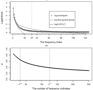
I now illustrate the asymptotic results using simulations. The sample size isn=1000, and the results reported are empirical means based on 5000 replications. First, consider the level shift process (3), withzt, ηt∼iid N(0,1)andπt∼iid B(1,5/n). Fig-ure1(a) depicts the log-periodograms as a function of the fre-quency index. An extra line, log(0.0015λ−j 2), is superimposed to highlight the slope of the periodogram whenj=o(n1/2). The figure is very informative. For very low frequencies, the slope of the log-periodogram is approximately−2,implyingd=1; forj>n1/2, the slope is basically zero. Thus nonuniformity is clearly present. I now impose the false restriction that the series are of true long memory and estimatef(λ)using the local Whit-tle likelihood with bandwidthm=n0.7. The fitted log-spectral densities are plotted in Figure1(a). The results again are quite informative, indicating that for very low frequencies,fˆ(λ) un-derestimates the slope of the log-periodogram and that for rel-atively higher frequencies, it does the opposite. The difference betweenˆf(λ)andIx(λ)provides an opportunity to test the null
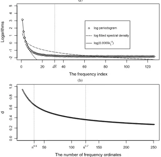
hypothesis. Figure1(b) reports the local Whittle estimates using different bandwidths,m, ranging betweenn1/3andn0.8. As pre-dicted by the theory, the estimates exceed 0.5 whenmis small, and they decrease substantially whenmis increased. Next, con-sider processes with smoothly varying trends of the form of (5). The series are generated using a simple polynomial trend function,h(x)=2x−4x2, with the errorszt being iid N(0,1). The analogous results are reported in Figure2(a) and (b). The findings are similar to the level-shift case and they confirm the asymptotic analysis. I also experimented with other low-order polynomial trend functions and found qualitatively similar re-sults.
These findings indicate that it is indeed possible to distin-guish between true and spurious long-memory, and that when doing so, it is important to consider frequencies both below and aboven1/2. In particular,m/n1/2→ ∞is necessary.
3. THE TEST STATISTIC
I now construct a test statistic for the null hypothesis thatxt is a long-memory process satisfying (1). This statistic is based on the local Whittle likelihood function given by (see Künsch 1987)
Q(G,d)= 1 m
m
j=1
logGλ−j 2d+ Ij Gλ−j 2d
, (6)
whereIj=Ix(λj)andmis some integer that is small relative to n. MinimizingQ(G,d)with respect toGleads to the profiled
(a)
(b)
Figure 1. (a) Spectral domain properties of processes with level shifts. (b) Local Whittle Estimates with differentmfor processes with level shifts.
(a)
(b)
Figure 2. (a) Spectral domain properties of processes with smooth trends. (b) Local Whittle estimates with differentmfor processes with smooth trends.
likelihood function, R(d) = logG(d)− 2m−1dm
j=1logλj, whereG(d)=m−1m
j=1λ2jdIj. The derivative ofR(d)is given by
∂R(d)
∂d =
2G0 √
mG(d) m −1/2
m
j=1 vj
I
j
G0λ−j2d −1
, (7)
wherevj=logλj−(1/m)mj=1logλjandG0is the true value of G. The term in the braces in (7) is the main ingredient of my test statistic. It is related to the LM statistic consid-ered by Robinson (1994). Under the null hypothesis and eval-uated atd0, it equalsm−1/2mj=1vj(Ijλ2jd0/G0−1), which, as shown by Robinson (1995b), satisfies a central limit theorem. Building on his result, I prove in Section 4 that the process m−1/2[mr]
j=1vj(Ijλj2d0/G0)−1) satisfies a functional central limit theorem and thus is uniformly Op(1)under the null hy-pothesis. Meanwhile, under the alternative hypothesis, the sum-mands in the preceding display do not have mean 0, and the quantity diverges [cf. the decomposition ofIx(λj)in the previ-ous section]. This motivates the following test statistic:
W= sup r∈[ε,1]
m
j=1 v2j
−1/2
[mr]
j=1 vj
I
j
G(ˆd)λ−j 2ˆd− 1
, (8)
wheredˆ is the local Whittle estimate ofd usingmfrequency components and ε is a small trimming parameter. Note that m−1m
j=1v2j →1, so that in principle,(
m
j=1v2j)−1/2could be
replaced bym−1/2. Using the former brings the exact size of the test closer to its nominal level, however.
Remark 2. The number of frequency ordinates, m, needs to satisfym/n1/2→ ∞to achieve good power and be less than n4/5to avoid bias when estimatingd. I use simulations to ex-amine the sensitivity of the results to such choices in Section6. It turns out thatm=n0.7seems to achieve a good balance be-tween size and power, and thus it is suggested in practice.
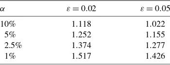
Remark 3. vjis unbounded forj=o(m). The introduction of trimming permits asymptotic approximations that are adequate even in small samples. Note that the test statistic and its criti-cal values are both decreasing functions ofε. In practice, if the sample size is small, sayn<500, then I suggest usingε=0.05. For larger samples, smaller trimmings can be used. I use simu-lations to evaluate the effect of different trimmings on the size and power of the test in Section6.
The test is a score-type test statistic. It does not require spec-ifying the form of the trend or the number or locations of the different regimes that occur under the alternative hypothesis. It inherits two desirable properties of the local Whittle estimator, which allows for non-Gaussianity and is more efficient than the GPH estimator (see Robinson1995b).
TheW test has some unique features compared with other similar tests reported in the literature. For example, Dolado, Gonzalo, and Mayoral (2005) proposed a test for the null hy-pothesis of fractional integration against the alternative hypoth-esis of short memory with a single structural break in the de-terministic component (a constant or a linear trend) that is
based on thet-statistic in an augmented Dickey–Fuller regres-sion. Mayoral (2010) considered a similar problem and pro-posed a likelihood ratio-type test statistic. Those two tests allow d>1/2 and are useful for detecting a single structural change. In contrast, theWtest is designed to detect a more general class of alternatives without requiring specification of the form of the trend or the number of breaks. Shimotsu (2006) proposed a Wald test that compares local Whittle estimates obtained from kequally sized subsamples, in line with the idea suggested by Lobato and Savin (1998). By choosingk>2, the test can han-dle multiple breaks. Shimotsu also proposed two tests based on thedth differenced series. I compare theWtest and Shimotsu’s tests using simulations in Section6.
4. ASYMPTOTIC PROPERTIES OF THE TEST
The following assumptions are imposed (as in Robinson 1995b). The folowing derivation makes heavy use of Robin-son’s results.
These assumptions allow for non-Gaussianity but preclude conditional heteroscedasticity. To allow for both features, I also consider an alternative set of conditions due to Shao and Wu (2007). Specifically, assume thatxtis generated by
(1−L)d(xt−E(x0))=ξt, t=0,±1,±2, . . . ,
where ξt =F(. . . ,e−1,e0, . . . ,et) with et being iid random variables andFbeing a measurable function such thatξtis well defined. The next assumption corresponds to assumptions 2.3, 2.4, and 2.6 of Shao and Wu (2007).
Assumption H. Assume that Assumption1is satisfied with β≥1 and that the following hold: (a)
The parameterβconcerns a particular property of the short-memory component ξt. Specifically, the condition β ≥1 im-plies that the component’s spectral density is differentiable at the origin. The cumulant condition in Assumption H(a)
is widely used in the time series literature. Andrews (1991, lemma 1) showed that it is implied by an α-mixing condition when ξt∈Lq withq>4. AssumptionH(b) quantifies the de-pendence ofξtone0by measuring the distance betweenξtand its coupled version ξk′, and can be verified for many nonlinear time series models. Shao and Wu (2007) showed that Assump-tion H(a) and (b) allow for ARFIMA(p,d,q)–GARCH(r,s) and ARFIMA(p,d,q)–EGARCH(r,s) processes provided that ξt∈Lqwithq>4. These processes haveβ=2. Note that As-sumption H(b) implies that the spectral density of ξt is con-tinuously differentiable over [−π, π], a property not required in Assumptions1–4. Also, AssumptionH(c) imposes stronger conditions onmthan does Assumption4. These are the prices we pay for allowing for conditional heteroscedasticity. Never-theless, simulation evidence presented in Section 6 indicates that the size of the test is insensitive to the choice of m, even when substantial conditional heteroscedasticity is present.
I first establish a uniform weak law of large numbers and a functional central limit theorem. These are needed for proving Theorem1and are also of independent interest.
Lemma 2. Let Qm(r)=m−1j[=mr1](Ij/(G0λ−j 2d0)). Under Assumptions 1–4 or Assumption H, Qm(r)→pr uniformly on[0,1]andm1/2(Qm(r)−r)⇒W(r), withW(r)the Wiener process on[0,1].
Theorem 1. Under Assumptions 1–4 or AssumptionH, as n→ ∞,
Theorem1is a result of the following first-order Taylor ap-proximation to (8):
The three terms inside the absolute value signs correspond to the three terms in the limiting distribution. Weak convergence is proved by first showing finite-dimensional convergence and then verifying tightness. The additional difficulty presented by AssumptionHis addressed using a martingale approximation technique developed by Wu and Shao (2007).
To simulate the limiting distribution, I approximate a Wiener process byn−1/2[nr]
i=1eiwithei∼iid N(0,1)andn=10,000,
Table 1. Asymptotic critical values of theWtest
NOTE: εis the trimming proportion.
and record 10,000 realizations ofW to tabulate its critical val-ues. The results are reported in Table 1, covering the cases whereε=0.02 and 0.05.
Remark 4. Lemma2 and Theorem 1 are useful for study-ing the distribution of other related test statistics. For example, instead of (8), a Cramer–von Mises-type statistic can be consid-ered:
Then it follows immediately that the limiting distribution is given by
The following result implies that the W test is consistent against the alternatives (3) and (5).
The assumption m/n1/2→ ∞is crucial for achieving con-sistency.P(ˆd> ǫ)→1 ensures that xt exhibits spurious long memory asymptotically. This is needed because we do not im-pose specific parametric assumptions on the form of the trend or level shifts and thus do not direct rule out the situation in which they are asymptotically negligible. To understand intu-itively what leads to this condition, note thatdˆsolves [cf. (7)]:
m−1 xt is a stationary short-memory process, then Ij is flat in j for both j∈ [1,j∗] and j∈ [j∗+1,m]. Thus dˆ will be close to 0 in large samples. If xt is affected by level shifts or trends, then the Ij in [1,j∗] will tend to increase, whereas those in[j∗+1,m]will stay flat; see (4) and Lemma1. Thus
ˆ
d needs to be positive to satisfy (9). It will be strictly pos-itive in large samples if the level shifts or trends are suffi-ciently pronounced. The conditionP(m−1m
j=1Ijλ2ˆjd> ǫ)→ 1 is a variance condition. To see this, consider a true long-memory process such as (2). Herem−1m
j=1Ijλ2jd0 converges in probability toσε2|B(1)|2/(2π|A(1)|2),the long-run variance of {B(L)A(L)−1εt}. Thus, these two conditions imply that xt mimics a long-memory process with strictly positive variance.
There is a connection between the foregoing results and those of Müller and Watson (2008, section 5). Those authors consid-ered a small number of frequencies and showed that detecting spurious long memory is very difficult, consistent with the find-ings in (4) and Lemma1. However, our Theorem2also shows that it is possible to construct useful tests if one is willing to consider frequencies beyondj=O(n1/2), at the cost of making additional assumptions about these frequencies.
Now consider the situation where both long memory and level shifts or smooth trends are present. Here there is spuri-ous long memory, because the presence of the latter tends to bias the estimate ofd0upward, thus spuriously increasing the apparent strength of long memory. I still consider the models (3) and (5) but withzt now being a true long-memory process. The next corollary shows the test is consistent against such al-ternatives.
Corollary 1. Suppose the processxt is generated by (3) or (5), but withzt being a true long-memory process, with mem-ory parameter d0, satisfying Assumptions 1–4 or Assump-tionH. Also assume that m/n1/2→ ∞, P(ˆd−d0> ǫ)→1, andP(m−1m
j=1Ijλj2ˆd> ǫ)→1 asn→ ∞withǫbeing some arbitrarily small constant. ThenW→p∞asn→ ∞.
The condition P(ˆd −d0 > ǫ)→1 implies that the pres-ence of level shifts or smooth trends spuriously increases the strength of long memory even asymptotically. The condition P(m−1m
j=1Ijλ2ˆjd> ǫ)→1 is again a variance condition, as in Theorem2. These two conditions imply thatxtmimics a long-memory process with a long-memory parameter greater thand0and strictly positive variance.
Remark 5. The foregoing approach corresponds to a “specif-ic-to-general” modeling approach, in which the simplest model (stationary long memory) is considered and tested, and addi-tional features are seen to be present if the test rejects the null hypothesis. This approach has some advantages. It is simple, with no need to specify the number of shifts or the form of the trend when conducting theWtest. The result is easy to interpret, because nonrejection implies that a long-memory model is ad-equate and rejection suggests that the series contains a spurious long-memory component. It gives clear modeling suggestions, that is, to build a long-memory model if theW test does not reject and incorporate trends or level shifts into the model if it does.
Now suppose that the W test rejects the null hypothesis. Then, to determine whether a true long-memory component is also present, it is necessary to reestimate the memory parameter after accounting for level shifts or a smooth trend.
Suppose that the presence of a smooth trend is conjectured, in which case the following procedures are useful. Beran and Feng
(2002) proposed a class of models (SEMIFAR models) that al-lows for a fractional component and a deterministic trend com-ponent. (I thank a referee for pointing this out.) The fractional component is specified as an ARFIMA process, and the trend component is modeled nonparametrically. The model can be estimated by combining parametric maximum likelihood esti-mation with kernel smoothing in an iterative fashion. Robinson (1997) and Hurvich, Lang, and Soulier (2005) considered semi-parametric estimation ofd in the presence of a smooth trend, with both the long-memory and the trend components specified nonparametrically. Both papers applied the local Whittle esti-mator. In the latter, the estimator was applied to the tapered, differenced series with a number of low frequencies trimmed from the estimator’s objective function. These studies provide confidence intervals fordˆ through which the evidence for long memory can be assessed.
For the level shift case, the following procedure can be considered. First, apply the method of Lavielle and Moulines (2000) to estimate the number and locations of the level shifts. Suppose thatkshifts are detected, resulting ink+1 exclusive subsamples. Second, apply the local Whittle estimator to each subsample to obtaindˆj(j=1, . . . ,k+1). Third, construct anF test ford1= · · · =dk+1=0.Under the hypothesis thatdj=0 and some additional assumptions—most importantly, that the level shifts are not too small (formally, their magnitudes stay-ing nonzero and fixed asn→ ∞)—dˆj have the usual asymp-totic distribution (as in Robinson 1995b) and are asymptoti-cally independent for different values ofj. Thus theFtest has a χ2(k+1)-limiting distribution. A rejection would then suggest that long memory is present after accounting for level shifts.
5. A FINITE–SAMPLE CORRECTION TO CONTROL SIZE
Although the short-memory dynamics do not enter the as-ymptotic distribution, they still may have a significant impact in small samples. In what follows, I propose a “prewhitening” pro-cedure that reduces the short-memory component while main-taining the same limiting distribution for the test. This proce-dure involves estimating a low-order ARFIMA model and fil-tering the series using the estimated autoregressive and moving average coefficients.
Step 1. Estimate an ARFIMA(p,d,q)model forp,q=0,1. Determine the order using the Akaike information criterion (AIC). Let μˆ =n−1n
i=1xt, and let aˆ1 and bˆ1 be the esti-mated autoregressive and moving average coefficients. Restrict the values ofaˆ1andbˆ1to lie strictly within the unit interval to ensure stationarity and invertibility, that is,−1+δ≤ ˆa1,bˆ1≤ 1−δ, withδbeing some small constant greater than 0. In sim-ulations and empirical applications, setδ=0.01.
Step 2.Computex∗t =(1− ˆa1L)(1+ ˆb1L)−1(xt− ˆμ). Explic-itly, letx1∗=x1− ˆμandx∗t =(xt− ˆμ)−tk−=11(−ˆb1)k−1(aˆ1+ ˆ
b1)(xt−k− ˆμ)fort>1. Usex∗t instead ofxtto constructW. In Step 1, the time domain Gaussian likelihood is used for constructing the AIC. In simulations and empirical applica-tions, it is computed using thefracdiff package in R, which im-plements the method of Haslett and Raftery (1989). The fore-going procedure does not affect the null limiting distribution, provided that Assumptions2andHare strengthened slightly.
Assumption F. (a) If Assumption2holds, then assume fur-ther thatαj=O(j−1/2−c)withc>0 asj→ ∞. (b) If Assump-tionHholds, then assume further thatξt satisfies a geometric moment contraction (GMC) condition with order q>4; that is, letξk∗=F(. . . ,e′−1,e′0, . . . ,ek−1,ek), withe′−j(j=0,1, . . .) being independent copies ofe−j. Assume thatξk−ξk∗q<Cρk for someC<∞, 0< ρ <1, and all positive integersk.
Assumption F(a) ensures that the square summability con-dition in Assumption2 is satisfied after filtering. It allows for stationary ARFIMA(p,d,q)models. AssumptionF(b) ensures that Assumption Hcontinues to hold after filtering. It allows for ARFIMA(p,d,q)–GARCH(r,s) and ARFIMA(p,d,q)– EGARCH(r,s) models. (See Shao and Wu2007for other mod-els satisfying GMC conditions.)
Corollary 2. Assume thatxtsatisfies the same conditions as in Theorem 1, with the additional requirement that Assump-tionFholds. Then theW test constructed usingx∗t has the same null limiting distribution as in Theorem1.
I do not assume that the true DGP is an ARFIMA process; rather I just use it as a reasonable approximation to the series so that some short-memory dynamics can be removed. I have proposed using ARFIMA(p,d,q) model withp,q≤1 as the basis for prewhitening. This is motivated by a host of research documenting that low-order ARFIMA models provide good ap-proximations to many processes considered in economics and finance. For example, Andersen et al. (2003) studied the log-realized volatility of the Deutschmark/Dollar and Yen/Dollar spot exchange rates and showed that an AFRIMA(1,d,0) ap-proximation performs quite well compared with other station-ary time series models. Deo, Hurvich, and Yi (2006), Koop-man, Jungbacker, and Hol (2005), and Christensen and Nielsen (2007) studied other volatility series and reached similar con-clusions. Note that μˆ can be replaced by estimated seasonal dummies. The procedure remains asymptotically valid.
6. SIMULATIONS FOR FINITE–SAMPLE PROPERTIES
This section examines the size and power properties of the W test using simulations, and compares this test with five test statistics in the literature. The first of these tests is due to Ohanissian, Russell, and Tsay (2008), given by ORT= (TDˆ)′(TT′)−1(TDˆ), where Dˆ =(ˆd(m1), . . . ,dˆ(mM)), where
ˆ
d(mj) is the GPH estimate of d at aggregation level mj, T is an(M−1)×Mmatrix of constants, andis defined by their equation (3). Following Ohanissian, Russell, and Tsay (2008), the aggregation levels are 2j−1withj=1, . . . ,M. Constrained by the sample size, I setM=4. The number of frequency ordi-nates used for each GPH estimate is the square root of the length of each (temporally aggregated) series. The second test is the mean-tdtest of Perron and Qu (2010). Letdˆa,cdenote the log-periodogram estimate ofdwhenc[na]frequencies are used, and lettd(a,c1;b,c2)=
24c1[na]/π2(ˆda,c1− ˆdb,c2). Then mean-td is defined as the average of thetd(1/3,c1;1/2,1)tests for c1∈ [1,2]. Its limiting distribution is not available. Following Perron and Qu (2010), a parametric bootstrap procedure is used
to compute relevant critical values. Specifically, for a given se-ries, an ARFIMA(1,d,1)model is estimated, and then the null distribution of the test is simulated using this as the DGP. Per-ron and Qu also considered a sup-td test, which performs very similar to the mean-tdtest in the present simulations and thus is omitted to save space. The remaining three test statistics are due to Shimotsu (2006). TheWctest compares estimates ofdfrom kequally sized subsamples. I setk=4,following the sugges-tion of Shimotsu (2006). Theημ andZt tests apply the KPSS and Phillips–Perron test to thedth differenced series. For these three tests, the parameterdis estimated using the local Whittle likelihood withm=4[(n0.7)/4]. Results are obtained using the Matlab code provided by Shimotsu.
For all local Whittle-based tests (W, ημ,Wc, andZt),dˆ is obtained by minimizing the objective function (6) over d∈ [−1/2,1]. Note that this interval is greater than that stated in Assumption1; however, this does not affect the test’s null limit-ing distribution, and can deliver tests with better size properties whend0is close to 0.5 by avoiding the boundary issue. All tests are constructed by first applying the finite-sample correction de-scribed in the previous section, except for the mean-tdtest. Be-cause the latter uses a bootstrap procedure to generate critical values, the finite-sample correction is irrelevant. The data are generated using thefracdiff package designed for the R envi-ronment. All results are based on 10,000 replications.
To evaluate the size of the test, I consider models with pa-rameter values that are typical in financial applications. The aforementioned studies, as well as others, suggest thatd typ-ically takes values between 0.30 and 0.45. Thus I setd=0.4 and consider the following specifications:
• DGP 1. ARFIMA(0,d,0):(1−L)0.4xt=et.
• DGP 2. ARFIMA(1,d,0): (1 −a1L)(1−L)0.4xt =et, wherea1=0.4 and 0.8.
• DGP 3. ARFIMA(0,d,1): (1 −L)0.4xt =(1 +b1L)et, whereb1=0.4 and 0.8.
• DGP 4. ARFIMA(2,d,0):(1−a1L)(1−a2L)(1−L)0.4× xt=et, wherea1=0.5 anda2=0.3.
• DGP 5. xt =zt+ηt, where (1−L)0.4zt=et and ηt ∼ iid N(0,var(zt)).
• DGP 6. (1 −L)0.4xt =ut with ut =σtet, σt2 =1 + 0.10u2t−1+0.85σt2−1.
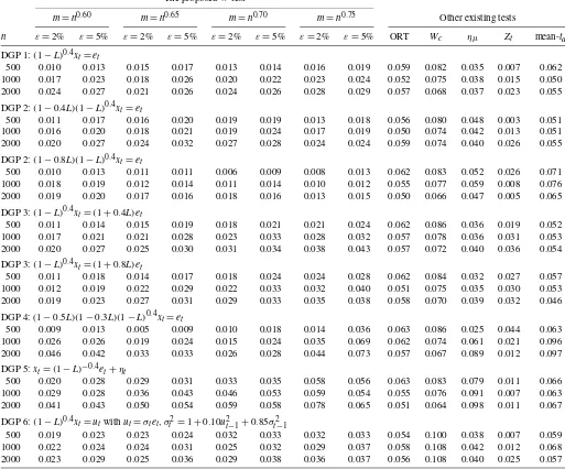
In all cases,et∼iid N(0,1). DGP 1 corresponds to the ideal sit-uation for local Whittle estimation. DGP 2, DGP 3, and DGP 4 contain substantial short-memory components. Because DGP 4 is not a subcase of ARFIMA(1,d,1)models, it is used to il-lustrate the effectiveness of the finite-sample correction. DGP 5 consists of a fractionally integrated process affected by mea-surement errors. Such a specification is relevant for applications to realized volatility. The variance of the measurement error is set equal to the variance of theztcomponent, following the sim-ulation design of Bandi and Perron (2006). DGP 6 exhibits con-ditional heteroscedasticity. For each DGP, I consider three sam-ple sizes,n=500, 1000, 2000. These are similar to the sample sizes in the empirical applications given in Section7.
Table2presents empirical rejection frequencies at a 5% nom-inal level. The size of the W test is fairly stable across dif-ferent sample sizes, DGPs, and values ofmandε. Overall, it appears to be conservative, but with a slight tendency toward
overrejection whenm=n0.75 for DGP 4 and DGP 5. The ORT test exhibits the best size properties. TheWc test of Shimotsu (2006) tends to overreject the null hypothesis, with a maximum rejection frequency of 0.108 for DGP 6. Other tests have de-cent sizes. I repeated the analysis using unfiltered series, and found that the finite-sample correction had no effect on ORT, had only a slight effect onWc, and significantly improved the W,ημ, and Zt tests, especially for DGPs 2, 4, and 5. For ex-ample, for DGP 2 witha1=0.8 andn=500, the rejection fre-quencies would be 0.352 for theW test (ε=0.02,m=n0.70), 0.000 for theημtest and 0.593 for theZttest if the finite-sample correction were not used. The size does not improve whennis increased to 2000, indicating that the correction is indeed quite effective.
For power properties, I consider six alternative models. The first five models are the same as those presented by Ohanissian, Russell, and Tsay (2008). The sixth model contains a smooth but nonmonotonic trend, for which parameter values are chosen to makedˆclose to 0.4.
1. Nonstationary random level shift: yt =μt +εt, μt = μt−1+πtηt,πt∼iid B(1,6.10/n),εt∼iid N(0,5),ηt∼ iid N(0,1).
2. Stationary random level shift: yt=μt+εt, μt =(1− πt)μt−1 + πtηt, πt ∼ iid B(1,0.003), εt and ηt ∼ iid N(0,1).
3. Markov switching with iid regimes: yt ∼iid N(1,1) if st=0 andyt∼iid N(−1,1)if st=1, with state transi-tion probabilitiesp10=p01=0.001.
4. Markov switching with GARCH regimes:rt=√htεtand ht=1+2st+0.4r2t−1+0.3ht−1, whereεt∼iid N(0,1), st=0,1, andp10=p01=0.001.yt=logrt2.
5. White noise with a monotonic deterministic trend:yt = 3t−0.1+εt,εt∼iid N(0,1).
6. White noise with a nonmonotonic deterministic trend: yt=sin(4πt/n)+εt,εt∼iid N(0,3).
The sample size, n, studied varies between 500 and 9000, and I set m=n0.70. Other specifications are the same as be-fore. Table 3 reports size-unadjusted power at a 5% nominal level, with bold numbers denoting the highest power among all tests. The results are encouraging. For models 1–4 and 6, the power of the W test with ε=0.02 is the highest among all tests oncen reaches 3000. The power difference is often sub-stantial, particularly for models 2–4 and 6. The power of ORT, mean-td, andZt, is generally much lower. Note that Ohanissian, Russell, and Tsay (2008) showed that the power of their test is 1 with a sample size of 610,304. Thus their test is more suit-able for very large sample sizes, which may be availsuit-able when analyzing high-frequency data. Forn=9000, I also tried to in-crease the number of aggregation levels toM=8 for the test of Ohanissian, Russell, and Tsay (2008). The rejection frequen-cies for the six processes are 0.46, 0.20, 0.11, 0.21, 0.24, and 0.23, respectively. The ημ and Wc tests of Shimotsu (2006) have merit; theημtest is very powerful for detecting monotonic
trends, a property inherited from the KPSS test. Their power is quite low under DGPs 2, 3, and 4, however. Thus the W test performs the best overall, in the sense that it has decent power against a wide range of alternatives for sample sizes typical in financial applications.
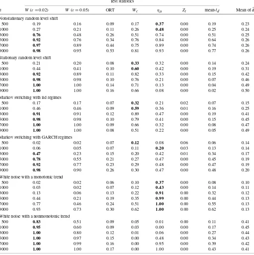
Table 2. Empirical size at 5% nominal level The proposedWtest
m=n0.60 m=n0.65 m=n0.70 m=n0.75 Other existing tests
n ε=2% ε=5% ε=2% ε=5% ε=2% ε=5% ε=2% ε=5% ORT Wc ημ Zt mean-td
DGP 1:(1−L)0.4xt=et
500 0.010 0.013 0.015 0.017 0.013 0.014 0.016 0.019 0.059 0.082 0.035 0.007 0.062 1000 0.017 0.023 0.018 0.026 0.020 0.022 0.023 0.024 0.052 0.075 0.038 0.015 0.050 2000 0.024 0.027 0.021 0.026 0.024 0.026 0.028 0.029 0.057 0.068 0.037 0.023 0.055 DGP 2:(1−0.4L)(1−L)0.4xt=et
500 0.011 0.017 0.016 0.020 0.019 0.019 0.013 0.018 0.056 0.080 0.048 0.003 0.051 1000 0.016 0.020 0.018 0.021 0.019 0.024 0.017 0.019 0.050 0.074 0.042 0.013 0.051 2000 0.020 0.027 0.024 0.032 0.027 0.028 0.024 0.024 0.059 0.074 0.040 0.026 0.055 DGP 2:(1−0.8L)(1−L)0.4xt=et
500 0.010 0.013 0.011 0.011 0.006 0.009 0.008 0.013 0.062 0.083 0.052 0.026 0.071 1000 0.018 0.019 0.012 0.014 0.011 0.014 0.010 0.012 0.055 0.077 0.059 0.008 0.076 2000 0.019 0.020 0.017 0.016 0.018 0.016 0.013 0.015 0.050 0.066 0.047 0.005 0.065 DGP 3:(1−L)0.4xt=(1+0.4L)et
500 0.011 0.014 0.015 0.019 0.018 0.021 0.021 0.024 0.062 0.086 0.036 0.019 0.052 1000 0.017 0.021 0.021 0.028 0.023 0.033 0.028 0.032 0.057 0.078 0.036 0.031 0.053 2000 0.020 0.027 0.025 0.030 0.031 0.034 0.038 0.043 0.057 0.072 0.040 0.036 0.054 DGP 3:(1−L)0.4xt=(1+0.8L)et
500 0.011 0.018 0.014 0.017 0.018 0.024 0.024 0.028 0.062 0.084 0.032 0.027 0.057 1000 0.012 0.019 0.022 0.029 0.022 0.033 0.032 0.040 0.051 0.075 0.035 0.030 0.053 2000 0.019 0.023 0.027 0.031 0.029 0.033 0.035 0.038 0.058 0.070 0.039 0.032 0.046 DGP 4: (1−0.5L)(1−0.3L)(1−L)0.4xt=et
500 0.009 0.013 0.005 0.009 0.010 0.018 0.014 0.036 0.063 0.086 0.025 0.044 0.063 1000 0.026 0.026 0.019 0.024 0.015 0.024 0.035 0.069 0.062 0.074 0.061 0.021 0.096 2000 0.046 0.042 0.033 0.033 0.026 0.028 0.044 0.073 0.057 0.067 0.089 0.012 0.097 DGP 5:xt=(1−L)−0.4et+ηt
500 0.020 0.028 0.029 0.031 0.033 0.035 0.058 0.056 0.063 0.083 0.079 0.011 0.066 1000 0.029 0.028 0.036 0.043 0.046 0.053 0.059 0.054 0.055 0.076 0.091 0.007 0.063 2000 0.041 0.043 0.050 0.054 0.059 0.058 0.078 0.065 0.051 0.064 0.098 0.011 0.067 DGP 6:(1−L)0.4xt=utwithut=σtet, σt2=1+0.10u2t−1+0.85σt2−1
500 0.019 0.023 0.023 0.024 0.032 0.033 0.032 0.033 0.054 0.100 0.038 0.007 0.059 1000 0.022 0.024 0.024 0.031 0.025 0.032 0.029 0.037 0.058 0.108 0.042 0.012 0.068 2000 0.023 0.029 0.025 0.036 0.029 0.038 0.036 0.037 0.056 0.108 0.040 0.025 0.057
NOTE: εis the trimming proportion. ORT: the test of Ohanissian, Russell, and Tsay (2008);Wc, ημandZt: tests of Shimotsu (2006); mean-td: the test of Perron and Qu (2010); the
mean-tdtest is constructed using unfiltered series.
Finally, the results show that a large trimming (ε=5%) may lead to a nonnegligible loss in power. Note that financial ap-plications typically involve samples of a few thousand observa-tions. In such cases, based on these limited simulation results, ε=2% seems to achieve a good balance in terms of size and power and thus is suggested in practice.
7. APPLICATIONS
I apply theWtest to three time series for which empirical ev-idence of long memory has been documented: (a) monthly tem-perature for the northern hemisphere for the years 1854–1989, (b) monthly U.S. inflation rates from January 1958 to December 2008, and (c) realized volatility for Japanese Yen/US dollar spot exchange rates from December 1, 1986 to June 30, 1999. TheW test usesm=n0.70unless stated otherwise. Other specifications are the same as before. The results of all tests are summarized in Table4.
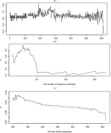
The temperature series, obtained from the work of Beran (1994, pp. 257–261), contains 1632 observations [Figure3(a)]. The local Whittle estimate is 0.33 usingm=n0.70. TheW test is significant at the 1% level for bothε=0.02 andε=0.05. To obtain some further insight, local Whittle estimates using differ-ent numbers of frequencies can be considered:n1/3≤m≤n4/5. These estimates are shown in Figure3(b) as a function ofm. The results are very informative, demonstrating that when a small number of frequencies is used, the estimate exceeds 0.5, and that the estimate decreases significantly as more frequen-cies are included. This finding is consistent with the presence of level shifts or smooth trends, but inconsistent with station-ary fractional integration [see Figures 1(b) and 2(b)]. Figure 3(c) provides more evidence. It reports memory parameter esti-mates using observations up tonb,withnbranging between 300 and 1632. The estimates vary substantially, again suggesting the presence of nonstationarity in the sample. Among the other tests,ημandWcrejects at 1% level, whereas the remainder do
Table 3. Finite sample power of the tests at a 5% nominal level Test statistics
n W(ε=0.02) W(ε=0.05) ORT Wc ημ Zt mean-td Mean ofdˆ
Nonstationary random level shift
500 0.19 0.16 0.09 0.17 0.37 0.00 0.19 0.23 1000 0.27 0.21 0.11 0.26 0.48 0.00 0.25 0.24
3000 0.76 0.48 0.26 0.51 0.74 0.00 0.51 0.25 5000 0.92 0.76 0.34 0.76 0.84 0.00 0.64 0.26 7000 0.97 0.89 0.44 0.75 0.89 0.00 0.74 0.26
9000 0.98 0.95 0.53 0.81 0.93 0.00 0.77 0.26 Stationary random level shift
500 0.21 0.20 0.08 0.33 0.32 0.00 0.14 0.24
1000 0.44 0.41 0.10 0.60 0.42 0.00 0.19 0.31 3000 0.92 0.89 0.11 0.82 0.33 0.00 0.15 0.42
5000 0.98 0.98 0.10 0.76 0.21 0.00 0.07 0.46 7000 1.00 1.00 0.14 0.71 0.13 0.00 0.04 0.49 9000 1.00 1.00 0.16 0.66 0.08 0.00 0.02 0.50
Markov switching with iid regimes
500 0.17 0.17 0.07 0.32 0.21 0.02 0.07 0.15 1000 0.46 0.46 0.09 0.59 0.36 0.01 0.16 0.25
3000 0.91 0.91 0.12 0.89 0.47 0.00 0.19 0.41 5000 0.98 0.98 0.10 0.79 0.41 0.00 0.15 0.45
7000 1.00 1.00 0.09 0.66 0.32 0.00 0.08 0.47 9000 1.00 1.00 0.08 0.51 0.22 0.00 0.05 0.49 Markov switching with GARCH regimes
500 0.02 0.02 0.07 0.12 0.08 0.06 0.06 0.14
1000 0.06 0.05 0.07 0.11 0.20 0.03 0.13 0.14 3000 0.47 0.23 0.15 0.20 0.42 0.01 0.34 0.17
5000 0.78 0.55 0.21 0.27 0.47 0.00 0.45 0.19 7000 0.92 0.77 0.23 0.29 0.48 0.00 0.47 0.19
9000 0.98 0.90 0.26 0.30 0.47 0.00 0.48 0.20 White noise with a monotonic trend
500 0.02 0.02 0.06 0.10 0.37 0.00 0.08 0.10 1000 0.03 0.02 0.07 0.12 0.43 0.00 0.14 0.11
3000 0.13 0.06 0.13 0.22 0.91 0.00 0.32 0.12 5000 0.44 0.21 0.19 0.35 0.99 0.00 0.44 0.13
7000 0.77 0.46 0.24 0.51 1.00 0.00 0.55 0.13 9000 0.93 0.73 0.30 0.62 1.00 0.00 0.62 0.13
White noise with a nonmonotonic trend
500 0.83 0.51 0.09 0.05 0.01 0.00 0.11 0.41 1000 0.95 0.60 0.09 0.03 0.00 0.00 0.17 0.45 3000 1.00 0.80 0.12 0.01 0.06 0.00 0.27 0.44
5000 1.00 0.97 0.15 0.00 0.48 0.00 0.34 0.43 7000 1.00 0.99 0.16 0.00 0.95 0.00 0.39 0.42
9000 1.00 1.00 0.17 0.00 1.00 0.00 0.43 0.41
NOTE: ε: the trimming proportion. ORT: the test of Ohanissian, Russell, and Tsay (2008);Wc, ημandZt: tests of Shimotsu (2006); mean-td: the test of Perron and Qu (2010); the
mean-tdtest is constructed using unfiltered series.
Table 4. Test statistics values for the three time series
Series W(ε=0.02) W(ε=0.05) ORT Wc ημ Zt mean-td
Temperature 2.09∗∗ 2.09∗∗ 1.67 11.55∗∗ 1.56∗∗ 0.93 0.31 (7.82, 11.35) (7.82, 11.35) (0.44, 0.71) (−2.92,−3.46) (1.51, 2.15) Inflation 1.51∗ 1.46∗∗ 1.82 16.34∗∗ 0.45∗ −0.62 −1.11
(7.82, 11.35) (7.82, 11.35) (0.44, 0.71) (−2.92,−3.46) (1.56, 2.23) Yen/$ volatility 0.41 0.37 0.15 2.18 0.19 −1.30 0.01
(7.82, 11.35) (7.82, 11.35) (0.44, 0.70) (−2.85,−3.41) (1.54, 2.20)
NOTE: * and ** denote significance at 5% and 1% level. The critical values of theWtest are reported in Table1. Other relevant critical values (at 5% and 1% level) are included in parentheses for reference. Note that the critical values ofημ,Zt, and mean-tdare model-dependent.
(a)
(b)
(c)
Figure 3. Results for the northern hemisphere temperature series. (a) The series: 1854–1989. (b) Memory parameter estimates with different numbers of frequency ordinates (m). (c) Memory parameter estimates using different subsamples.
not reject even at 5% level. This is consistent with the simu-lation evidence thatημ andWc have relatively higher power among the remaining five tests.
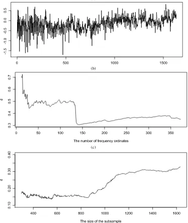
The inflation series was constructed from the consumer price index for all urban consumers and all items (series SA0, season-ally unadjusted, available from the Bureau of Labor Statistics). It contains 612 observations and is plotted in Figure4(a). The local Whittle estimate is 0.33 usingm=n0.70. The W test is significant at the 5% level whenε=0.02 and at the 1% level whenε=0.05. Figure4(b) and (c) reveal qualitatively similar findings as shown in Figure3, presenting evidence against the null hypothesis of stationary long memory. Among the other tests, Wc rejects at the 1% level,ημ barely rejects at the 5%
level, and the remainder do not reject.
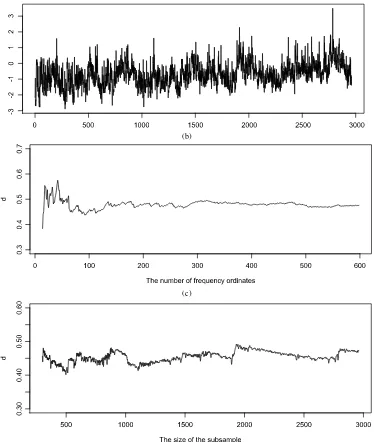
The realized volatility series was constructed using 5-minute returns for the Yen/Dollar spot rate, obtained from Olsen and
Associates. The series was constructed following the same pro-cedure used by Andersen et al. (2003). Specifically, I first ob-tained the daily realized variances by summing the squared 5-minute returns, then applied the logarithm transformation to ob-tain log-realized volatility. The weekends and holidays were dropped in accordance with the method of Andersen et al. (2003), leaving a sample of 2960 observations. The local Whit-tle estimate is 0.47 using m=n0.70. The W test equals 0.41 whenε=0.02 and 0.37 whenε=0.05, both of which are well below the 10% critical values. Figure5(b) and (c) show that the memory parameter estimates remain stable with changes in the number of frequency ordinates or sample size. Other tests lead to the same conclusion. I repeated the analysis using 30-minute returns and found qualitatively similar results.
The foregoing findings suggest that the evidence for sta-tionary long memory might not be as strong as is often per-ceived. They also suggest that more research is needed to
(a)
(b)
(c)
Figure 4. Results for the U.S. inflation rate series. (a) The series: 1958–2008. (b) The memory parameter estimates with different numbers of frequency ordinates (m). (c) The memory parameter estimates using different subsamples.
derstand the nonlinear and nonstationary aspects of the relevant processes.
8. CONCLUSION
I have considered the issue of distinguishing between true and spurious long memory. I began by comparing the spectral domain properties of stationary long-memory processes with short-memory processes containing level shifts or smoothly varying trends, then proposed a simple test statistic based on the derivatives of the profiled local Whittle likelihood function. The limiting distribution under the null hypothesis was derived using the theory of empirical processes. Simulations showed that the test has decent size and power properties. The test was applied to three time series for which empirical evidence for long memory has been documented. The result of this empirical
exercise suggests that the evidence for stationary long memory might not be as strong as is often perceived.
APPENDIX A: PROOF OF MAIN RESULTS
This appendix contains proofs for Lemma1and Theorem1. Proofs for Lemma2, Theorem2, and Corollaries1 and2are provided in the supplementary appendix.
Proof of Lemma1
The proof is a direct extension of Künsch (1986, p. 1026). Consider
Ih(λj)= 1 2πn
n
t=1
h(t/n)cos(λjt)
2
+ 1
2πn
n
t=1
h(t/n)sin(λjt)
2
.
(a)
(b)
(c)
Figure 5. Results for the Yen/Dollar spot exchange rate series. (a) The log realized volatility: 1986–1999. (b) Memory parameter estimates with different numbers of frequency ordinates (m). (c) Memory parameter estimates using different subsamples.
Forj∈ {1,2, . . . ,[n/2]},
n
t=1
h(t/n)cos(λjt)
≤ n−1
t=1
h((t+1)/n)−h(t/n)
t
s=1
cos(λjs)
≤ n−1
t=1
h((t+1)/n)−h(t/n) max
1≤t≤n
t
s=1
cos(λjs)
≤12 n−1
t=1
h((t+1)/n)−h(t/n)
π
λj + 1
≤(n−2n1)C
π
λj+ 1
for some 0<C<∞,
where the first inequality uses summation by parts and
n
s=1
cos(λjs)=0,
the third inequality follows from t
s=1cos(λjs)=sin((t+ 1/2)λj)/(2 sin(λj/2))−1/2, and the fourth inequality is due to Lipschitz continuity ofh(·). Similarly,|n
t=1h(t/n)sin(λjt)| ≤ (n−n1Cπ )λ−j 1. Hence,Ih(λj)=O(n−1λ−j 2).
Proof of Theorem1
The proof comprises three steps:
Step 1[Represent the statistic as a quantity linear in(ˆd−d0)]. Apply a first-order Taylor expansion,
Ym(r,d)ˆ =m−1/2 sion can be rewritten as
m−1/2 G0
Next, consider (A.1). Adding and subtracting
the term in the curly brackets in (A.1) can be rewritten as m−1vjmk=1λ2˜kdIk−m−1ms=1vsλ2˜sdIs. Thus,
Lemma B.3 in the supplementary appendix shows that
1 Step 2(Prove finite-dimensional convergence). Consider the first term in (A.4). Because G0/G(d0)→p 1, it suffices to Then it suffices to show
n
First, the asymptotic normality of (n
t=1zt,rs)s=1,...,p follows
from theorem 2 of Robinson (1995b) and theorem 3.1 of Shao and Wu (2007). Second, for 0≤r1≤r2≤1, Robinson 1995b, p. 1645). The second term converges to
r1
0 (1+logs)2dsby Lemma B.1. Thus (A.6) holds.
Consider the second term in (A.4). Because of Lemma B.7,
m−1/2
Also, because of Lemma B.1,m−1[mr]
Thus this can be analyzed in the same way as for the second term. The details are omitted.
Step 3(Prove tightness). I follow Nielsen (2004) and use the-orem 13.5 of Billingsley (1999); that is, I show that for everym andr1≤r≤r2, is finite, is nondecreasing, and satisfies
lim
Proofs and Additional Simulation Evidence: A pdf file con-taining (1) additional simulation evidence for finite sample properties of the test, and (2) proofs for Lemma 2, The-orem 2, Corollaries 1 and 2 and some auxiliary lemmas. (Supplementary-appendix.pdf)
ACKNOWLEDGMENTS
The author thanks Serena Ng (the past editor), Jonathan Wright (the editor), an associate editor, and two anonymous referees for detailed and valuable suggestions. He also thanks Benoit Perron, Pierre Perron, Morten Nielsen, Aaron Smith and participants at 2009 CIREQ Time Series Conference for useful suggestions, and Adam McCloskey and Yohei Yamamoto for detailed comments on a previous draft that improved the pre-sentation.
[Received June 2009. Revised July 2010.]
REFERENCES
Andersen, T., Bollerslev, T., Diebold, F. X., and Labys, P. (2003), “Modeling and Forecasting Realized Volatility,”Econometrica, 71, 579–626. [423,429,
433]
Andrews, D. W. K. (1991), “Heteroskedasticity and Autocorrelation Consistent Covariance Matrix Estimation,”Econometrica, 59, 817–858. [427] Bandi, F. M, and Perron, B. (2006), “Long Memory and the Relation Between
Implied and Realized Volatility,”Journal of Financial Econometrics, 4, 636–670. [430]
Bartlett, M. S. (1955),An Introduction to Stochastic Processes With Special Reference to Methods and Applications, London: Cambridge University Press. [423]
Beran, J. (1994),Statistics for Long-Memory Processes, Chapman & Hall. [431]
Beran, J., and Feng, Y. (2002), “SEMIFAR Models—A Semiparametric Ap-proach to Modelling Trends, Long-Range Dependence and Nonstationar-ity,”Computational Statistics & Data Analysis, 40, 393–419. [429] Billingsley, P. (1999),Convergence of Probability Measures(2nd ed.), New
York: Wiley. [437]
Christensen, B. J., and Nielsen, M. Ø. (2007), “The Effect of Long Memory in Volatility on Stock Market Fluctuations,”Review of Economics and Statis-tics, 89, 684–700. [429]
Deo, R., Hurvich, C., and Yi, L. (2006), “Forecasting Realized Volatility Us-ing a Long-Memory Stochastic Volatility Model: Estimation, Prediction and Seasonal Adjustment,”Journal of Econometrics, 131, 29–58. [423,429] Ding, Z., Engle, R. F., and Granger, C. W. J. (1993), “A Long Memory Property
of Stock Market Returns and a New Model,”Journal of Empirical Finance, 1, 83–106. [423]
Dolado, J. J., Gonzalo, J., and Mayoral, L. (2005), “What Is What?: A Simple Time-Domain Test of Long-Memory vs. Structural Breaks,” working paper, Universidad Carlos III de Madrid. [423,426]
Fox, R., and Taqqu, M. S. (1986), “Large Sample Properties of Parameter Esti-mates for Strongly Dependent Stationary Time Series,”The Annals of Sta-tistics, 14, 517–532. [423]
Geweke, J., and Porter-Hudak, S. (1983), “The Estimation and Application of Long Memory Time Series Models,”Journal of Time Series Analysis, 4, 221–238. [423]
Grenander, U., and Rosenblatt, M. (1957),Statistical Analysis of Stationary Time Series, New York: Wiley. [423]
Haslett, J., and Raftery, A. E. (1989), “Space–Time Modelling With Long-Memory Dependence: Assessing Ireland’s Wind Power Resource” (with discussion),Applied Statistics, 38, 1–50. [429]
Hurvich, C., Lang, G., and Soulier, P. (2005), “Estimation of Long Memory in the Presence of a Smooth Nonparametric Trend,”Journal of the American Statistical Association, 100, 853–871. [429]
Ibragimov, I. A. (1963), “On Estimation of the Spectral Function of a Stationary Gaussian Process,”Theory of Probability and Its Applications, 8, 366–401. [423]
Kokoszka, P., and Mikosch, T. (1997), “The Integrated Periodogram for Long Memory Processes With Finite or Infinite Variance,”Stochastic Processes and Their Applications, 66, 55–78. [423]
Koopman, S. J., Jungbacker, B., and Hol, E. (2005), “Forecasting Daily Vari-ability of the S&P 100 Stock Index Using Historical, Realised and Im-plied Volatility Measurements,”Journal of Empirical Finance, 12, 445– 475. [429]
Künsch, H. R. (1986), “Discriminating Between Monotonic Trends and Long-Range Dependence,”Journal of Applied Probability, 23, 1025–1030. [425,
434]
(1987), “Statistical Aspects of Self-Similar Processes,” inProceedings of the First World Congress of the Bernoulli Society, Vol. 1, Utrecht: VNU Science Press, pp. 67–74. [425]
Lavielle, M., and Moulines, E. (2000), “Least-Squares Estimation of an Un-known Number of Shifts in a Time Series,”Journal of Time Series Analysis, 21, 33–59. [429]
Lobato, I. N., and Savin, N. E. (1998), “Real and Spurious Long-Memory Prop-erties of Stock-Market Data,”Journal of Business & Economic Statistics, 16, 261–268. [427]
Mayoral, L. (2010), “Testing for Fractional Integration versus Short Memory With Trends and Structural Breaks,” working paper, Universitat Pompeu Fabra. [423,427]
Müller, U. K., and Watson, M. (2008), “Testing Models of Low Frequency Vari-ability,”Econometrica, 76, 979–1016. [423,428]
Nielsen, M. Ø. (2004), “Local Empirical Spectral Measure of Multivariate Processes With Long Range Dependence,”Stochastic Processes and Their Applications, 109, 145–166. [423,437]
Ohanissian, A., Russell, J. R., and Tsay, R. S. (2008), “True or Spurious Long Memory? A New Test,”Journal of Business & Economic Statistics, 26, 161–175. [423,429-432]
Perron, P., and Qu, Z. (2010), “Long-Memory and Level Shifts in the Volatility of Stock Market Return Indices,”Journal of Business & Economic Statis-tics, 28, 275–290. [423,424,429,431,432]
Robinson, P. M. (1994), Efficient Tests of Nonstationary Hypotheses,”Journal of the American Statistical Association, 89, 1420–1437. [426]
(1995a), “Log Periodogram Regression of Time Series With Long Range Dependence,”The Annals of Statistics, 23 1048–1072. [423,424]
(1995b), “Gaussian Semiparametric Estimation of Long Range De-pendence,”The Annals of Statistics, 23, 1630–1661. [423,424,426,427,429,
436]
(1997), “Large-Sample Inference for Nonparametric Regression With Dependent Errors,”The Annals of Statistics, 25, 2054–2083. [429] Shao, X., and Wu, W. B. (2007), “Local Whittle Estimation of Fractional
Integration for Nonlinear Processes,”Econometric Theory, 23, 899–929. [423,427,429,436]
Shimotsu, K. (2006), “Simple (but Effective) Tests of Long Memory versus Structural Breaks,” working paper, Queen’s University. [423,427,430-432] Wu, W. B., and Shao, X. (2007), “A Limit Theorem for Quadratic Forms and
Its Applications,”Econometric Theory, 23, 930–951. [427]