Full Terms & Conditions of access and use can be found at
http://www.tandfonline.com/action/journalInformation?journalCode=ubes20
Download by: [Universitas Maritim Raja Ali Haji] Date: 11 January 2016, At: 22:59
Journal of Business & Economic Statistics
ISSN: 0735-0015 (Print) 1537-2707 (Online) Journal homepage: http://www.tandfonline.com/loi/ubes20
A General Multivariate Threshold GARCH Model
With Dynamic Conditional Correlations
Francesco Audrino & Fabio Trojani
To cite this article: Francesco Audrino & Fabio Trojani (2011) A General Multivariate Threshold
GARCH Model With Dynamic Conditional Correlations, Journal of Business & Economic Statistics, 29:1, 138-149, DOI: 10.1198/jbes.2010.08117
To link to this article: http://dx.doi.org/10.1198/jbes.2010.08117
Published online: 01 Jan 2012.
Submit your article to this journal
Article views: 205
View related articles
A General Multivariate Threshold GARCH Model
With Dynamic Conditional Correlations
Francesco AUDRINO
Department of Economics, Institute of Mathematics and Statistics, University of St. Gallen, CH-9000 St. Gallen, Switzerland (francesco.audrino@unisg.ch)
Fabio TROJANI
University of Lugano and Swiss Finance Institute, CH-6900 Lugano, Switzerland (fabio.trojani@usi.ch)
We introduce a new multivariate GARCH model with multivariate thresholds in conditional correlations and develop a two-step estimation procedure that is feasible in large dimensional applications. Optimal threshold functions are estimated endogenously from the data and the model conditional covariance ma-trix is ensured to be positive definite. We study the empirical performance of our model in two applica-tions using U.S. stock and bond market data. In both applicaapplica-tions our model has, in terms of statistical and economic significance, higher forecasting power than several other multivariate GARCH models for conditional correlations.
KEY WORDS: Dynamic conditional correlations; Multivariate GARCH models; Tree-structured GARCH models.
1. INTRODUCTION
In this article, we present a new multivariate GARCH model with dynamic conditional correlations (DCC) that extends pre-vious approaches by admitting multivariate thresholds in the conditional volatilities and correlations of multivariate time se-ries. This extension allows us to account for rich asymmetric effects and dependencies of conditional volatilities and correla-tions that are often encountered, for instance, in financial real data applications. As in the classicalEngle(2002) DCC model, our model estimation is numerically feasible in large dimen-sions. Moreover, the positive definiteness of the conditional co-variance matrix is ensured in a natural way by the structure of the model. Finally, thresholds in volatilities and correlations of our model are not fixed ex ante, but are estimated from the data together with all other parameters in the model.
To define the threshold function in our model, we extend the tree-structured state space partition inAudrino and Bühlmann (2001) to a setting with multivariate thresholds in volatilities and correlations. As shown inAudrino and Trojani(2006) and Audrino(2006), the tree-structured threshold construction can incorporate a potentially large number of multivariate regimes in univariate settings in a parsimonious way. In this article, we study a multivariate model with a potentially large num-ber of tree-structured thresholds in volatilities and correlations and we develop a feasible estimation strategy that can be ap-plied to estimate the model in large dimensional applications as well. The threshold construction is obtained using a binary tree in which each terminal node defines local GARCH-type dynamics for volatilities and correlations over a partition cell of the multivariate state space. The estimation is performed by a simple two-step procedure that estimates the number and struc-ture of the underlying thresholds together with the parameters of the local GARCH dynamics for volatilities and correlations. The optimal threshold structure is identified by solving a high-dimensional model selection problem based on the Schwarz Bayesian information criterion (BIC).
We estimate our model in two distinct applications to U.S. stock and bond market data and focus on the explanatory power for future conditional correlations, comparing the results with a set of competing models in the literature:Engle’s (2002) DCC model,Ledoit, Santa-Clara, and Wolf’s (2003) flexible multi-variate GARCH model, andPelletier’s (2006) regime switch-ing dynamic correlations (RSDC) model. As in our model, the DCC and the RSDC models can be estimated by a two-step pro-cedure that separates the estimation of the conditional volatility and correlation dynamics. In order to measure, where possi-ble, the additional forecasting power for correlations, we es-timate these models using a set of univariate tree-structured GARCH dynamics for volatility identical to the one in our model. The flexible multivariate GARCH model cannot be timated by a two-step estimation procedure. Therefore, the es-timated volatility dynamics are different from the dynamics of our model. Our model differs from the others in the way it spec-ifies the correlation dynamics. The DCC and the flexible mul-tivariate GARCH models are single-regime models for correla-tions and the RSDC model specifies a very simple regime struc-ture for conditional correlations. By contrast, our setting can account parsimoniously for GARCH-type dynamics and multi-variate conditional correlation thresholds without ex ante fixing the structure and the number of thresholds.
Using our tree-structured GARCH-DCC model, we empiri-cally study the relative importance of GARCH and threshold ef-fects in the conditional correlation dynamics of U.S. stock and bond returns. The conditional volatility functions of U.S. stock returns exhibit GARCH and threshold features, but conditional correlations depend on a piecewise constant threshold function. By contrast, we find both threshold and GARCH effects for the correlation process of stock and government bond returns, with
© 2011American Statistical Association Journal of Business & Economic Statistics January 2011, Vol. 29, No. 1 DOI:10.1198/jbes.2010.08117
138
estimated thresholds that are functions of lagged stock and bond returns. In all applications, the estimated tree-structured parti-tion of the state space improves the forecasting power for con-ditional correlations relative to the other multivariate GARCH models. Out-of-sample improvements are, in most cases, sta-tistically and economically significant based on different cri-teria recently proposed in the literature including the test for superior predictive ability (SPA) introduced byHansen(2005), the model confidence set approach ofHansen, Lunde, and Na-son(2003), and the economic measure of volatility and correla-tion timing ability for portfolio allocacorrela-tion inEngle and Colac-ito(2006) andBandi, Russell, and Zhu(2008). These findings highlight the importance of flexible multivariate threshold and GARCH structures for forecasting the conditional correlation of stock and bond markets.
In this article, we develop a multivariate GARCH model for variances and correlations, which has good forecasting power and which can be estimated exclusively from informa-tion on multivariate returns. A completely different approach can instead formulate a dynamic model for realized volatili-ties and correlations, using information from intraday returns when available, in order to produce even more accurate fore-casts; see, for example,Andersen et al.(2003) orAudrino and Corsi (2009). This empirical strategy produces very good re-sults in univariate settings. However, its extension to the multi-variate context is not straightforward because of the difficulty of accurately estimating realized correlations under nonsynchro-nous intraday returns. It was shown that this problem can pro-duce high efficiency losses in estimating high-dimensional real-ized variance covariance matrices; see, for example, Barndorff-Nielsen et al.(2008) orChiriac and Voev(2009). Solving this important issue is a crucial topic of ongoing research.
Section2presents our tree-structured GARCH-DCC model and Section3describes the two-step estimation procedure that can be applied to estimate it. Section4presents our empirical study of the conditional correlation dynamics of U.S. stock and bond returns. Section5summarizes the main results and con-cludes.
2. THE MODEL
We consider a multivariate stochastic process(Xt)t∈Z with
values inRd:
Xt=Dtǫt, (2.1)
whereDt:=diag[σ1,t, . . . , σd,t]andσi,tis the conditional
stan-dard deviation of theith component ofXtat timet−1.(ǫt)t∈Z
is a zero-mean process inRd with components having a unit conditional standard deviation by construction. To simplify the notation, conditional means of Xt were set to zero in
Equa-tion (2.1). The condiEqua-tional covariance matrix ofǫtat timet−1 is denoted byRt. Therefore, we obtain the following standard
factorization of the conditional covariance matrix ofXt:
covt−1(Xt)=DtRtDt. (2.2)
Our tree-structured DCC-GARCH model parameterizes the conditional volatility matrix Dt and the conditional
correla-tion matrixRtby means of two parametric threshold functions.
Each diagonal element of Dt is modeled as a univariate
tree-structured threshold GARCH(1,1)-model, as in Audrino and Bühlmann(2001) andAudrino and Trojani(2006). The condi-tional correlation matrixRtis modeled according to a threshold
DCC-type model described in more detail in the following.
2.1 Tree-Structured Model forDt
LetXt,jbe thejth component ofXt. In principle, the
thresh-olds in the volatility dynamics of Xt,j may depend on all
components of Xt−1. For simplicity of exposition, let us
as-sume that they are functions of (Xt−1,1,Xt−1,j). Let Pj =
{R1,j, . . . ,Rk
j,j}be a partition of the state spaceG:=R 2×R+
of(Xt−1,1,Xt−1,j, σt2−1,j):
Pj=R1,j, . . . ,Rk
j,j
,
kj
s=1
Rs,j=G, Ri,j∩Rs,j= ∅ (i=s).
Given a partition cellRi,j, we specify the local conditional
vari-ance dynamics ofXt,jonRi,jas a GARCH(1,1)model.
There-fore, the threshold functionσt2,jtakes the form
σt2,j=
kj
i=1
(αij+βijX2t−1,j+γijσt2−1,j)
×I[(X
t−1,1,Xt−1,j,σt2−1,j)∈Ri,j], (2.3) whereI[·]is the indicator function andθ1,jis the parameter
vec-tor
θ1,j= {αij, βij, γij;i=1, . . . ,kj}.
To completely specify the conditional variance function in Equation (2.3), we have to define the class of partitions Pj
that are admissible in our tree-structured model. The first as-sumption is thatPj is composed of rectangular cellsRi,j,i=
1, . . . ,kj, so that they can be easily parameterized by a set of
multivariate thresholds for (Xt−1,1,Xt−1,j, σt2−1,j). The second
assumption is that the potential partition cells satisfy a hierar-chical structure that can be mapped one-to-one on a so-called binary tree by means of an iterative statistical procedure. In this way, the multivariate threshold function in the model follows the structure of a binary treeTj in which every terminal node
represents a particular regime.
In constructing the binary tree, it is first tested whether a thresholdd1can split the whole state space into two
rectangu-lar partition cells representing two different volatility regimes. In this case,d1defines the first node on the binary tree and the
first two partition cells represent the two stems associated with the first node. This tree-structure is preferred with respect to a model with no variance–covariance thresholds if the implied improvement in goodness of fit is large enough. In the second step, it is checked whether one of the two cells identified from the first step can be further split into two rectangular subcells by an additional threshold d2. The decision on which subcell
can be further split is again based on a comparison of the im-provement in the implied goodness of fit. Thresholdd2defines
a second node on the binary tree. Two subcells are associated with this node that define two new stems of the tree and two
further volatility subregimes. Such a procedure is iterated until a maximal tree and a maximal number of variance–covariance regimes are obtained. See the following for additional details on the model construction and the estimation procedure. Details on the interpretation of binary trees in the context of volatility models are provided inAudrino and Trojani(2006).
Consider, for example, a model with three regimes, i.e., two thresholds, and partitioning cellsR1,j,R2,j,R3,jof the form:
R1,j= {Xt−1,j≤d1},
R2,j= {Xt−1,j>d1andXt−1,1≤d2},
R3,j= {Xt−1,j>d1andXt−1,1>d2},
where the parametersd1,d2define the two multivariate
thresh-olds in the model. In this case, R1,j is associated with a
regime of low conditioning values Xt−1,j. R2,j corresponds
to a regime with higher conditioning values of Xt−1,j, but
low values ofXt−1,1. Finally, R3,j implies a regime in which
both conditioning valuesXt−1,1 andXt−1,j are large. For each
component Xt,j, estimation of Equation (2.3) is achieved by a
high-dimensional model selection problem that determines the optimal number and the structure of the relevant thresholds (and hence the partition cells) inPj. Details of this estimation
pro-cedure for univariate tree structured GARCH(1,1)models are given inAudrino and Bühlmann(2001) andAudrino and Tro-jani(2006, section 2.3).
2.2 Tree-Structured Model forRt
Givenθ1= {θ1,j:j=1, . . . ,d}, let
ǫt=Dt(θ1)−1Xt
and
Rt=corrt−1(Xt)=covt−1(ǫt).
We modelRtby means of a tree-structured model in which
con-ditional correlations satisfy an Engle(2002)-type local DCC model across several multivariate thresholds. In order to keep the model tractable, we assume that thresholds in the Rt
dy-namics depend onǫt−1only via the average
ρt−1= 1
d(d−1)
u=v
ǫt−1,uǫt−1,v,
of the cross products of the component ofǫt−1. Intuitively, this
choice allows us to account for asymmetric effects in condi-tional correlations as a function of particular lagged process re-alizationsXt−1and specific movements in average lagged
con-ditional correlation shocksρt−1.
To define the parametric threshold functionRtin our model,
let P = {R1, . . . ,Rw} be a partition of the state space G:=
Rd+1 of (Xt−1, ρt−1). We consider the following family of
functional forms forRt
Rt=
andQis, as in the classicalEngle(2002) DCC model, the un-conditional covariance matrix of the residualsǫt. Given a fixed
partitionP, the parameter vector
θ2= {ci, φi, λi,vech(Q);i=1, . . . ,w}, (2.7)
completely parameterizes the threshold function defining the conditional correlation function in Equation (2.4).
Since for anyi=1, . . . ,w, the local model forQitsatisfies an
Engle(2002) DCC-type dynamics, positive definiteness of the resulting threshold model forRtis easily implied by the model
structure under the above conditions on the model parameters. WhenP= {G}, i.e., the partition is trivial, we obtain theEngle (2002) DCC model by settingc1= · · · =cw=1. Therefore,
this model is nested in our model. Moreover, by settingφi=
λi=0 fori=1, . . . ,w, we can writeRtas
whereR is a fixed d-dimensional correlation matrix. In this case, we obtain a piecewise constant correlation matrix defined by a multivariate threshold function over the partition P. In
contrast to the RSDC model inPelletier(2006), this particular subcase of our model can account for a flexible description of multiple multivariate regimes in correlations because the num-ber and the structure of the regimes in the estimated model does not have to be fixed from the beginning. Finally, whenφi>0
orλi>0 fori=1, . . . ,wandPis not a trivial partition, by
set-tingc1= · · · =cw=1 we obtain a tree-structured DCC model
locally satisfying Engle’s DCC dynamics over the distinct par-titioning cellsRi.
As for the univariate tree-structured volatility dynamics of the last section, we need to define the class of admissible parti-tionsPfor our correlation function. Again, the only restriction
we put onP is that it is composed of rectangular partition cells.
Consistent with our assumptions, these partition cells are delim-ited by a set of multivariate thresholds for(Xt−1, ρt−1). In order
to construct such rectangular partition cells, we make use of a binary tree in which every terminal node represents a cellRi.
Estimation of the threshold function in the correlation dynam-ics in Equation (2.4) is achieved by a high-dimensional model selection procedure that determines the optimal number and the structure of the relevant thresholds in the underlying partition. This model selection scheme is not computationally feasible if applied directly to the multivariate time series(ǫtǫ′
t)t∈Z. A
nat-ural way to reduce estimation complexity is to notice that the partitionP is identical to the one implied by a corresponding
tree-structured univariate model for the time series(ρt)t∈Z.
In-(Rit). Therefore, the tree-structured model
ρt=Et−1(ρt)+ηt, (2.10)
where(ηt)t∈Zis a martingale difference process andEt−1(ρt)
is given by Equation (2.9), defines a univariate tree-structured process forρtbased on the same partitionP as in the
correla-tion dynamics in Equacorrela-tion (2.4). It follows that we can exploit the univariate model in Equation (2.10) to estimate the thresh-old structure in Equation (2.4). In particular, we can develop a model selection procedure for selecting the optimal threshold structure in the correlation dynamics. The simplest dynamics arise in the piecewise constant case
Et−1(ρt)=
whereRuvis theuvcomponent of the correlation matrixRin the constant dynamics in Equation (2.8). This piecewise-constant function is the optimal one that was estimated in our applications to the U.S. equity market in Section 4.1. More generally, forc1= · · · =cw=1 andλi, φi>0, i=1, . . . ,w,
we can also encompass the univariate dynamics ofρt that are
consistent with a tree-structured DCC model of the form in Equation (2.4) for correlations. This threshold structure is the one we estimate in our application of Section 4.2where we model the correlation between Treasury bond and stock returns. Model selection across this class of potential threshold func-tions forEt−1[ρt]is performed using the BIC information
cri-terion. Once the partition P in Equation (2.10) is estimated
the parameter in Equation (2.7) of the multivariate correla-tion dynamics can be estimated using a multivariate condicorrela-tional pseudo-likelihood for ǫt in which the selected partition P is
held fixed. The next section provides additional details on the estimation procedure used to estimate our tree-structured DCC model.
3. ESTIMATION OF THE TREE–STRUCTURED DCC MODEL
Estimation of our tree-structured model is accomplished in two steps. In the first step, an estimate of the volatil-ity process Dt is obtained by performing d estimations of
the univariate tree-structured conditional volatility dynamics
σt,1(θ1,1), . . . , σt,d(θ1,d)implied by the specification in
Equa-tion (2.3). The resulting point estimateDt:=Dt(θ1)is used to
compute the estimated scaled residuals
ǫt:=D−t 1Xt. (3.1)
The scaled residualsǫtare used in the second step of our
proce-dure to estimate the tree-structured conditional correlation dy-namics in Equation (2.4).
3.1 Estimation of Tree-Structured Univariate GARCH-Dynamics
Estimation of thedtree-structured univariate volatility func-tions in Equation (2.3) is achieved by a high-dimensional model selection problem that determines the optimal structure of the relevant thresholds in any partitionPjof the univariate
volatil-ity dynamics in Equation (2.3),j=1, . . . ,d.
In the first step, the largest univariate tree-structured GARCH model is estimated for any j=1, . . . ,d, given a fixed maxi-mal numberMj of possible thresholds in Equation (2.3). This
first step delivers a maximal possible partitionPmax
j of the
rele-vant state spaceGin the univariate volatility dynamics in Equa-tion (2.3).
In the second step, a tree-structured model selection proce-dure for nonnested models is applied that selects the optimal subpartition Pj ⊂Pmax
j out of the maximal one. Model
se-lection is performed according to the BIC information crite-rion implied by a conditionally Gaussian log-likelihood for any process coordinateXt,j,j=1, . . . ,d. The resulting optimal
tree-structured volatility model minimizes the BIC information cri-terion across all tree-structured subpartitions ofPmax
j . The
com-plete algorithm used to estimate univariate tree-structured GARCH(1,1) models is given in Audrino and Bühlmann (2001) andAudrino and Trojani(2006).
The construction of the largest partition Pmax
j proceeds as
follows: We first fix a maximal numberMj+1 of partition cells
in the tree. Because of the tree-structured construction ofPmax
j ,
this first step implies a maximal numberMj+1 of conditional
volatility regimes (i.e., the number of terminal nodes in the bi-nary tree). A parsimonious specification of the maximal num-berMjof thresholds ensures a statistically and computationally
tractable model dimension. Moreover, it avoids (over) fitting an overly flexible model dynamics, which will result in a poor out-of-sample forecasting power. For any coordinate axis of the multivariate state space that has to be split, we search for mul-tivariate thresholds over grid points that are empiricalα quan-tiles of the data along the relevant coordinate axis. We fix the empirical quantiles asα=i/mesh,i=1, . . . ,mesh−1, where mesh determines the fineness of the grid on which we search for multivariate thresholds. We choose mesh=8 because, as was shown in different empirical studies in the literature, this value leads to reliable forecasting results. The partition of the state space G=Rd×R+ into a maximal number of M cells Rleft,Rright is further partitioned with a second
thresh-old d2 and a second component indexι2, in the same way as
previously. We then iterate this procedure. For the mth itera-tion step, we specify a new pair(dm, ιm), which defines a new
thresholddm for the coordinate indexed byιm and an existing
partition cell that is going to be split into two subcells. For a
new pair(d, ι)∈R× {1, . . . ,d+1}refinement of an existing partitionP(old)is obtained by pickingRj∗∈P(old)and splitting
it as
Rj∗=Rj∗,left∪Rj∗,right. (3.2)
This procedure produces a new (finer) partition ofG, given by
P(new)= {Rj,Rj∗,left,Rj∗,right,j=j∗}. (3.3)
In this partition, the tuple (d, ι) describes a threshold d and a component index ι such thatRj∗,left= {(Xt−1, σ2
t−1)∈Rj∗; (Xt−1, σt2−1)ι ≤d}. Rj∗,right is defined analogously, with the
relation “>” instead of “≤.” The whole procedure finally de-termines a partitionPmax
j = {R1,j, . . . ,RMj+1,j}. This partition can be represented and summarized by a binary tree in which every terminal node represents a partition cell ofPmax
j . To
se-lect the specific threshold and component index(d, ι)in each it-eration step of the above procedure we optimize the correspond-ing conditional negative (pseudo) log-likelihood in the model.
3.2 Estimation of Tree-Structured DCC-Dynamics
In the first step, we estimate the optimal partitionPusing the
tree-structured model in Equation (2.10) forρt and the scaled estimated residualsǫt. In the second step, we fix the partition
P estimated for the univariate model in Equation (2.10), and
estimate the parameter θ2 in Equation (2.7) by a multivariate
pseudo-maximum likelihood estimator.
(i) Estimation of the univariate tree-structured model in Equation(2.10). Let
ρt=
u=v
ǫt−1,uǫt−1,v/[d(d−1)]. (3.4)
The following tree–structured model forρt is estimated; com-pare with Equation (2.10)
ρt=Et−1(ρt)+ηt, (3.5)
where(ηt)t∈Zis a martingale difference sequence and Et−1(ρt)=
w
i=1 ci
1
d(d−1)
u=v
ˆ
Ruvit
I[(X
t−1,ρt−1)∈Ri].(3.6)
In this equation,Rˆit denotes fori=1, . . . ,wa constant
corre-lation matrix when the tree-structured model for correcorre-lations implies a piecewise-constant correlation matrix. It then fol-lows in this case that the conditional mean ofρt is simply a piecewise-constant threshold function. More generally, for
c1= · · · =cw=1 and φi>0 orλi>0, where i=1, . . . ,w,
the local conditional correlation matrixRˆitis simply defined in
the same way asRitin Equations (2.5) and (2.6), but withǫˆt−1
replacingǫt−1in Equation (2.6).
We apply to the series ρt the same estimation procedure given in the last section for individual conditional variances. First, we estimate a largest univariate tree-structured model for
ρt, given a fixed maximal numberM of possible thresholds in Equation (2.10). In all our empirical applications, we fix the maximal number of candidate thresholds in Equation (2.10) at M =4. A tree-structured model selection procedure for
nonnested models is then applied that selects the optimal sub-partition P out of the maximal one. Model selection is
per-formed according to the BIC criterion implied by a condition-ally Gaussian pseudo log-likelihood forρt; see againAudrino and Trojani (2006, section 2.3), for details on this estima-tion procedure. In our empirical study, we find that this pro-cedure offers a simple and effective way to reduce the com-putational costs implied by the estimation of our multivariate tree-structured model. In particular, in the applications of Sec-tion4a piecewise-constant conditional correlation function is estimated for equity returns. However, local DCC-type struc-tures are found to better model the conditional correlations be-tween equity and bond returns.
(ii) Estimation of the tree-structured conditional correlation functionRt. In the second step of our estimation procedure, we
fix the partitionPestimated in step (i) and we estimate the
pa-rameter vectorθ2in Equation (2.7) by a pseudo-maximum
like-lihood estimatorθ2forθ2, under a Gaussian multivariate
condi-tional pseudo-likelihood forǫt. If in step (i) the optimal
thresh-old function does not imply piecewise-constant correlations, we estimate the matrixQin the dynamics in Equation (2.6) by do-ing correlation targetdo-ing, as proposed byEngle and Sheppard (2001) andPelletier(2006). If in step (i) a piecewise-constant correlation structure is selected, in the second step we estimate a piecewise constant correlation process of the form in Equa-tion (2.8). In such a case, we estimate the constant matrixRby doing correlation targeting in a rolling window of one year of data. The piecewise-constant correlation structure significantly reduces the number of parameters over which the likelihood function has to be maximized.
3.3 Consistency
Proofs of the consistency of our model selection procedure are very difficult to obtain for the case where the true model is in the class of tree-structured GARCH-DCC models. Analogously to the standard classification and regression trees (CART) pro-cedure introduced by Breiman et al. (1984), it is possible to prove theorems that study the behavior of the prevailing para-meter estimators when growing the tree. However, such results do not imply model selection consistency. Furthermore, it is quite unlikely that the “correct” generating process in our ex-ample and other similar ones with real data is indeed exactly a tree-structured model for volatilities and correlations. For this reason, it is more important to prove consistency of the estima-tors for the parameters of a tree-structured model under a model misspecification than it is to prove consistency of the model se-lection strategy under the assumption of a correctly specified, tree-structured model. Such consistency results can be found in Audrino and Bühlmann(2001). Based on these results, consis-tency of the two-step estimates(θ1,θ2)in the tree-structured DCC-GARCH model under a possible model misspecification can be derived in the standard way under mild regularity con-ditions; see, for instance,Newey and McFadden(1994). More-over, efficient estimates can be obtained by performing a further one-step Newton–Raphson estimation of the full likelihood, us-ing as startus-ing values the parameter estimates obtained from the two-step procedure (see, e.g.,Pagan 1986).
4. RESULTS
In this section we test the in-sample and out-of-sample ex-planatory power of our tree-structured GARCH-DCC (TreeDCC) model in two different applications involving the econometric analysis of U.S. stock and bond returns. We com-pare our model with several multivariate GARCH models that were recently proposed in the literature. Some of these models are nested in ours and can be estimated by a two-step estimation procedure:
• The CCC-GARCH model, as proposed by Bollerslev (1990); this model is nested in our model.
• The DCC-GARCH model, as proposed byEngle(2002); this model is nested in our model.
• The RSDC-GARCH model with switching regimes in conditional correlations, as proposed inPelletier (2006). This model is not formally nested in ours.
Since the individual volatility processes are estimated sep-arately from the correlation dynamics in these models, in our empirical study we can easily focus on the additional explanatory power for conditional correlations, which is the main topic of this article. To achieve this goal, we estimate volatility processes identical to those in our tree-structured DCC-GARCH setting. The volatility processes are all speci-fied as univariate tree-structured GARCH(1,1)processes. We also study the performance of our model relative to the flexible multivariate GARCH setting inLedoit, Santa-Clara, and Wolf (2003), which does not include thresholds in volatilities or cor-relations and is based on a more general correlation dynamics than the one implied by theEngle(2002) DCC model. There-fore, this model is not nested in our setting. Flexible multivari-ate GARCH models were shown byLedoit, Santa-Clara, and Wolf(2003) to describe the dynamics of stock returns quite ac-curately. Therefore, they are further natural competitors of our approach, especially in applications that study the multivariate dynamics of stock markets, as in our first empirical example.
To quantify and compare the in-sample and out-of-sample fit of the different models, we compute several goodness-of-fit sta-tistics for conditional covariances. Since the individual volatil-ity processes are identical for all but the flexible multivariate GARCH model, this comparison allows us to investigate the additional explanatory power of our model for explaining the correlation dynamics. We consider the following goodness-of-fit measures:
• The multivariate negative log-likelihood statistic (NL),
• The multivariate version of the classical mean absolute er-ror statistic (MAE), and
• The multivariate version of the classical mean squared er-ror statistic (MSE).
The last two performance measures require the specification of sensible values for the unknown true conditional covariance matrix. A powerful way of computing good proxies for this matrix is by means of the so-called realized covariance ap-proach, which is the natural multivariate version of the real-ized volatility approach proposed, among others, byAndersen et al.(2001, 2003) andBarndorff-Nielsen and Shephard(2001, 2002). We follow this approach in our two real data applica-tions, in which we collect tick-by-tick return data to compute
the realized covariance between returns using the methodology proposed in Corsi and Audrino (2007). Using such an accu-rate proxy for the unobservable conditional covariance matrix allows us to avoid possible misleading results implied by an un-fortunate choice of the loss function used to quantify the good-ness of fit, and therefore, a wrong ranking of the different mod-els under investigation; see Laurent, Rombouts, and Violante (2009) for more details. All estimated models also include a linear autoregressive conditional mean function modeled by a simple diagonal VAR(1)process.
The different statistics used to quantify the in-sample and out-of-sample goodness of fit in our empirical analysis are de-fined as follows (IS denotes in-sample and OS denotes out-of-sample):
IS-NL: −log-likelihood(Xn1;θ1,θ2),
OS-NL: −log-likelihood(Ynout
1 ;θ1,θ2),
where in the OS performance measures the expression
vt,ij(Yt1−1) is the ijth covariance prediction implied by our
out-of-sample dataYnout
1 = {Y1, . . . ,Ynout}at timet under the
parameter estimates obtained from the in-sample data Xn1= {X1, . . . ,Xn}.vt,ijis the realized covariance between the return
series i and j at time t. In all cases, a lower goodness-of-fit measure indicates a higher forecasting power of a model for conditional correlations.
To evaluate whether differences in performance among the models considered are statistically and/or economically signif-icant, we perform a series of tests recently proposed in the lit-erature. We investigate the statistical relevance of the improve-ments in forecasting accuracy of the TreeDCC model relative to the other approaches:
• We perform the superior predictive ability (SPA) test intro-duced byHansen(2005). This allows us to verify whether each of the models considered is significantly outper-formed by one (or more) of the alternatives.
• We construct a model confidence set (MCS) at the 5% and 10% confidence levels as proposed byHansen, Lunde, and Nason(2003). We introduce the MCS approach with the goal of characterizing the best subset of models out of a set of competing ones; see theAppendixfor more details about the MCS construction.
We also evaluate the alternative model specifications using an economic criterion. We apply the methodology suggested by West, Edison, and Cho(1993) andFleming, Kirby, and Ostdiek
(2001,2003) to quantify the economic benefit of different cor-relation forecasts in the context of a portfolio strategy based on volatility timing. Similarly to Engle and Colacito (2006) and Bandi, Russell, and Zhu(2008), we employ the variance com-ponent of an investor’s long-run mean–variance utility as a met-ric to quantify the economic differences between the alternative correlation (covariance) forecasts
AU=λ
2 1
nout
nout
t=1
(Rpt −Rp)2,
where the portfolio return at timetis given by
Rpt =Rf +w′t−1(Yt−RfId), t=1, . . . ,nout. Rp is the sample mean of the portfolio returns across the out-of-sample period and λ is a coefficient of risk aversion. As in Bandi, Russell, and Zhu (2008), we use three values of
λ=2,7,10. In the computation of the portfolio returns, Rf
is the risk-free rate, Id is a d×1 unit vector, and wt−1 is a d vector of portfolio weights obtained by solving the classi-cal mean–variance optimization problem at timet−1, given a fixed target return on the portfolio. In our real data applica-tions, we set Rf equal to the average value of the U.S. three-month rate in the out-of-sample period. In the mean–variance optimization, we use the one-step-ahead conditional covariance forecasts vˆt,ij(Yt1−1) obtained from the alternative
multivari-ate GARCH models under investigation. We can interpret the difference between the quantity AU implied by the TreeDCC model and each other model as the fee that an investor will be willing to pay to switch from correlation forecasts generated by each alternative model to those of the TreeDCC model. We also use the generalization of the Diebold–Mariano test for pairwise equal predictive ability (EPA) and the joint test introduced in Engle and Colacito(2006) to study the statistical significance of the differences in estimated economic gains. For details, see againEngle and Colacito(2006) andBandi, Russell, and Zhu (2008).
4.1 First Real Data Application: U.S. Equity Returns
We consider a multivariate time series of (annualized) daily log-returns for 10 U.S. stocks: Alcoa, Citigroup, Hasbro, Harley Davidson, Intel, Microsoft, Nike, Pfizer, Tektronix, and Exxon. Data are for the sample period between January 2, 2001 and De-cember 30, 2005, amounting to 1256 trading days. The source of the data is Tick Data, a division of Nexa Technologies, Inc. (see the webpage http:// www.tickdata.com). Using these tick-by-tick data, we construct realized covariances using the method inCorsi and Audrino(2007) and obtain the quantities
vt,ijneeded to compute our goodness-of-fit measures.
We split the sample into two subperiods. The first one con-sists ofn=752 trading days, from January 2, 2001 to Decem-ber 31, 2003. Data from this subperiod are used for in-sample estimation and performance evaluation. The second subperiod consists of the remaining nout=504 observations, up to
De-cember 30, 2005, and is used for out-of-sample performance evaluation.
We focus on differences in goodness of fit implied by the conditional correlation matrix dynamics under the different model settings. We estimate our model in two steps as follows.
First, we separately estimate the univariate conditional volatil-ity dynamics for each single return series and include as possi-ble conditioning variapossi-bles in the threshold definition (i) its es-timated conditional volatility and (ii) the first lag of all compo-nents in the multivariate return series. This threshold volatility structure proved to produce good empirical results in applica-tions of tree-structured GARCH models to financial data; see, for example,Audrino and Trojani(2006). This first step of the estimation procedure is kept identical for all models in which volatilities can be estimated separately from correlations: the CCC, the DCC, the RSDC, and our tree-structured DCC model. In this way, we ensure that differences in the goodness of fit of these models with respect to the estimated conditional covari-ance matrix dynamics are exclusively due to differences in the explanatory power with respect to conditional correlations. In the second step of our estimation procedure, we estimate pos-sible tree-structured thresholds and GARCH-type dynamics in conditional correlations. We include as possible conditioning variables for the definition of the threshold structure of con-ditional correlations (i) the first lag of the average concon-ditional correlation shocks across returns and (ii) the first lag of all com-ponents of our multivariate return series; see again Section2.2 for details.
4.1.1 Estimation Results. The estimation results of our TreeDCC-GARCH model for the 10-dimensional time series of U.S. stock returns introduced earlier are summarized in Table1. Table1, Panel A, highlights that, at most, two regimes are necessary to model the individual conditional variance dynam-ics accurately. The most important predictor variables impact-ing on the correspondimpact-ing threshold structures are the lagged re-turns of Microsoft and Harley Davidson. Microsoft and Harley Davidson are the largest stocks in our empirical example. Thus, the apparent influence of their lagged returns on estimated vari-ance covarivari-ance regimes is likely to proxy for the latent impact of the aggregate market return on the multivariate variance co-variance dynamics. The structure of the estimated conditional correlation dynamics in our model is summarized in Panel B of Table1. Similar to volatilities, the most important and sta-tistically significant predictor variable impacting on the thresh-old structure of conditional correlations is the lagged return of Harley Davidson. Moreover, the complete threshold structure of conditional correlations is characterized using only two fur-ther lagged stock returns, the returns of Alcoa and Intel (in de-scending order of statistical significance), implying four cor-relation regimes overall. The first regime is associated with simultaneously low (i.e., under the threshold values) lagged Harley Davidson and Alcoa returns. The second one arises for lagged, low Harley Davidson returns and for large Alcoa re-turns. The third regime is obtained for lagged low Intel returns and large Harley Davidson returns. Finally, the fourth regime is caused by contemporarily somewhat higher returns of Harley Davidson and Intel. An important difference between the esti-mated volatility and correlation dynamics is that the local cor-relation dynamics never exhibit GARCH-type effects across the different correlation regimes. In other words, conditional corre-lations are regime dependent but piecewise constant. The local average correlation levels in the different regimes are similar and vary from 0.897 to 0.962. However, we find that the BIC criterion increases significantly in all cases when incorporating
Table 1. Estimation results for a multivariate time series of 10 daily (annualized) U.S. stock returns (in %)
Panel A: Individual conditional variance structures
Series Regimes Optimal predictors
Alcoa 1 —
Citigroup 2 Microsoft
Hasbro 2 Harley Davidson
Harley Davidson 2 Harley Davidson
Intel 1 —
Microsoft 1 —
Nike 2 Exxon
Pfizer 2 Microsoft
Tektronix 2 Harley Davidson
Exxon 1 —
Panel B: Conditional correlation structure and parameters
Cond. corr. structure Cond. corr. parameters
Rk ck
Xt−1,Harley Davidson≤ −19.983 and 0.918
Xt−1,Alcoa≤ −3.553 (0.029)
Xt−1,Harley Davidson≤ −19.983 and 0.897
Xt−1,Alcoa>−3.553 (0.056)
Xt−1,Harley Davidson>−19.983 and 0.962
Xt−1,Intel≤ −15.016 (0.016)
Xt−1,Harley Davidson>−19.983 and 0.935
Xt−1,Intel>−15.016 (0.023) NOTE: Data are for the in-sample time period between January 2, 2001 and De-cember 31, 2003, consisting of 752 observations. Estimated individual conditional vari-ance structures (Panel A) and estimated conditional correlation structure and parameters (Panel B) are for the tree-structured GARCH-DCC model fit. Standard errors computed using 1000 model-based bootstrap replications are given in parentheses.
additional correlation regimes into the model. This finding is also supported by our out-of-sample tests on the model’s fore-casting power for correlations, which further indicate a clear superiority of our model over a CCC model with constant cor-relations.
4.1.2 Multivariate Performance Results. We now com-pare the accuracy of the conditional correlation predictions
implied by our model with those implied by the CCC, the DCC, the RSDC, and the flexible multivariate GARCH model. Since all models have the same individual volatility dynamics, with the sole exception being the flexible multivariate GARCH model, any difference in the goodness of fit for the forecasts of the return covariance matrix is due to a difference in the qual-ity of the forecasts for conditional correlations. In Table2, we present the goodness-of-fit measures defined in Section4 for the real data application to our 10-dimensional stock return se-ries.
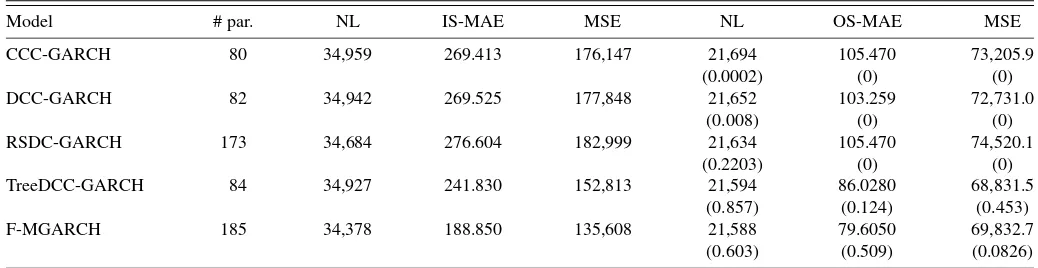
Our multivariate tree-structured model achieves the highest goodness of fit overall across the models with identical volatil-ity dynamics (TreeDCC, CCC, DCC, and RSDC models). The RSDC model achieves a better in-sample log-likelihood criterion, but it implies worse MAE and MSE criteria both in-sample and out-of-in-sample. Since the RSDC model has more than twice the number of parameters of the other models, we interpret this finding as evidence of over-fitting for this partic-ular model. The TreeDCC model’s better performance relative to CCC, DCC, and RSDC ranges between 0.5% and 17% de-pending on the goodness-of-fit measure applied. In compari-son with the flexible multivariate GARCH model, we find that the out-of-sample forecasting performance of the latter spec-ification is slightly better in two out of three cases, despite this model’s having more than double the number of parame-ters of ours. The heavy parameterization of the flexible mul-tivariate GARCH model can make it impracticable for set-tings that include dozens to hundreds of individual time series. Our TreeDCC model can produce flexible conditional covari-ance specifications combined with a sufficient degree of parsi-mony. This is why the TreeDCC model, like the CCC, DCC, and RSDC models, can be used to estimate the conditional variance–covariance dynamics of very high-dimensional time-series settings.
4.1.3 Statistical and Economic Significance of the Improve-ments. In this section, we provide additional evidence of the statistical and economic significance of the goodness-of-fit im-provements provided by our model. We focus first on the sta-tistical significance of improvements in conditional variance– covariance forecasts. To this end, we first compute Hansen
Table 2. Goodness of fit of different models for a multivariate time series of 10 daily (annualized) U.S. stock returns (in %)
U.S. equity returns: Goodness-of-fit results
Model # par. NL IS-MAE MSE NL OS-MAE MSE
CCC-GARCH 80 34,959 269.413 176,147 21,694 105.470 73,205.9
(0.0002) (0) (0)
DCC-GARCH 82 34,942 269.525 177,848 21,652 103.259 72,731.0
(0.008) (0) (0)
RSDC-GARCH 173 34,684 276.604 182,999 21,634 105.470 74,520.1
(0.2203) (0) (0)
TreeDCC-GARCH 84 34,927 241.830 152,813 21,594 86.0280 68,831.5 (0.857) (0.124) (0.453)
F-MGARCH 185 34,378 188.850 135,608 21,588 79.6050 69,832.7
(0.603) (0.509) (0.0826)
NOTE: Data are for the time period between January 2, 2001 and December 30, 2005, for a total of 1256 observations. The in-sample estimation period goes from the beginning of the sample to the end of 2003 (752 observations). NL, MAE, and MSE are multivariate versions of the standard univariate negative log-likelihood, the mean absolute error, and the mean squared error statistics. # par. reports the number of parameters estimated by the different models. For the out-of-sample performance measures,p-values of superior predictive ability (SPA) tests are reported in parentheses.
(2005) tests of superior predictive ability. In Table2,p-values of these tests are reported for each model and each out-of-sample performance measure under investigation.
Consistent with our previous results, the TreeDCC and flex-ible multivariate GARCH models are the only ones not signifi-cantly outperformed by any other model at the 5% significance level based on the MAE and MSE statistics. With respect to the negative log-likelihood statistic, the RDSC model is also not significantly outperformed by any other model at the 20% sig-nificance level. In this case, however, thep-values implied by TreeDCC and flexible GARCH models are even higher (above 85% and 60%, respectively). To formally characterize the set of models not significantly outperformed by other ones, we also computedHansen, Lunde, and Nason(2003) model con-fidence sets (MCS). Consistent with the previous findings for SPA tests, we find that the 5% MCS based on the OS-MAE and OS-MSE criteria using the range and semiquadratic statistics consist solely of the TreeDCC and flexible MGARCH mod-els. Ten percent MCS based on the OS-NL criterion include the TreeDCC, flexible MGARCH and RSDC models.
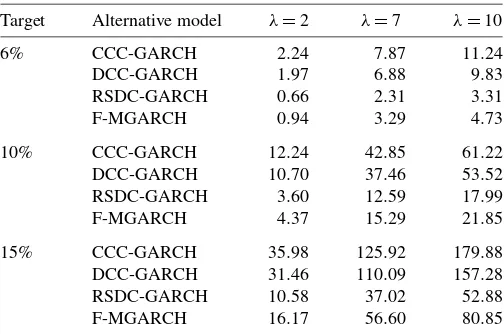
We now economically quantify the improvements implied by the different variance–covariance forecasts and compute the difference between the variance component of the average util-ityAUimplied by TreeDCC model and the one implied by each of the other models. Table3presents results for three levels of risk aversion parametersλ=2,7,10 and three target expected returns (6%, 10%, and 15%) for the mean variance optimal portfolio. The resulting difference between average utilities is shown as an annualized fee and the (annualized) risk-free rate is 3%.
The economic gains relative to CCC and DCC models range from about 1 to 180 basis points. The economically most im-portant gains arise for highly risk-averse investors (λ=10) and high target expected returns of 15%. Economically, very
Table 3. U.S. equity returns: Annualized fees (in basis points)
Target Alternative model λ=2 λ=7 λ=10
6% CCC-GARCH 2.24 7.87 11.24 DCC-GARCH 1.97 6.88 9.83 RSDC-GARCH 0.66 2.31 3.31 F-MGARCH 0.94 3.29 4.73
10% CCC-GARCH 12.24 42.85 61.22 DCC-GARCH 10.70 37.46 53.52 RSDC-GARCH 3.60 12.59 17.99 F-MGARCH 4.37 15.29 21.85
15% CCC-GARCH 35.98 125.92 179.88 DCC-GARCH 31.46 110.09 157.28 RSDC-GARCH 10.58 37.02 52.88 F-MGARCH 16.17 56.60 80.85
NOTE: The table contains the annualized fees (in basis points) that a conditional mean-variance investor with absolute risk-aversion parameterλ=2, 7, and 10 will be willing to pay to perform volatility timing using the one-step-ahead conditional correlation and covariance forecasts from the TreeDCC model (benchmark model) versus those obtained using the CCC, DCC, RSDC, and the flexible MGARCH models. The portfolio weights are obtained by minimizing the one-step-ahead conditional variance forecast of a portfolio containing 10 U.S. stocks and the risk-free asset for a given target expected return on the portfolio. The annual risk-free rate is set to be equal to 3%. Data are for the out-of-sample time period beginning in January 2004 and ending in December 2005, for a total of 504 daily observations.
small gains arise for low risk aversion (λ=2) and a target expected return of 6%. Consistent with our previous findings, economic gains are clearly smaller relative to RSDC and flex-ible MGARCH models. In this case, for a high risk aversion
λ=10 and a target expected return of 15%, they are 52 and 81 basis points, respectively. We can use a Diebold–Mariano-type test and the joint test proposed inEngle and Colacito(2006) to test the statistical significance of these differences. Similarly to Bandi, Russell, and Zhu(2008), we find that these differences are not significant at the 5% significance level.
Overall, these results provide evidence that economically and statistically significant differences in variance–covariance fore-casts of our TreeDCC model are likely to arise with respect to the CCC and DCC models, whereas with respect to the RSDC and flexible GARCH models, such differences are less likely.
4.1.4 Sensitivity Analysis. To investigate the robustness of our findings, it is useful to study the sensitivity of results to moderate changes in the structure of the estimated TreeDCC model. We perform this task along several dimensions.
First, we investigate whether moderate changes in the es-timated location and threshold parameters of the conditional correlation process imply significantly different out-of-sample performances given a fixed tree-structure. Overall, the result-ing effect on the out-of-sample performance relative to the esti-mated TreeDCC model is economically small. The largest im-pact arises by modifying the location parameterc4in the fourth
regime (of±1 standard error) or the first threshold parameterd1
(to the nearest possible threshold value in the positive and neg-ative directions). However, the changes in forecasting accuracy are typically smaller than the changes in MAE and MSE ob-served for the CCC, DCC, RDSC, and flexible GARCH mod-els.
Second, we investigate whether moderate changes in the tree-structure of the estimated TreeDCC model imply significantly different out-of-sample performances. We consider the second, third, and fourth best (in-sample) TreeDCC models estimated according to the procedure described in Section3. Once again, the good forecasting performance of our TreeDCC modeling approach relative to other models seems to be quite robust across various similar choices of the parameters and threshold structure in the model. More detailed results of this sensitivity exercise are available from the authors upon request.
4.2 Second Real Data Application: U.S. Stock Index and Bond Returns
We consider a two-dimensional time series of (annualized) daily log-returns for the U.S. S&P500 stock index and the U.S. 30-year Treasury bond. The time period under investigation goes from January 3, 1996 to October 30, 2003 and contains 1899 trading days. The data are provided byTick Data. As in the previous section, we exploit the tick-by-tick data to con-struct the series of realized volatilities and covariances between stock index and bond returns. As before, for forecasting evalu-ation purposes we split the sample in two subperiods. The first subperiod consists ofn=1219 trading days and goes from Jan-uary 3, 1996 to December 29, 2000. The second subperiod con-sists of the last three years of data (nout=680 observations).
Table 4. Estimation results for a two-dimensional time series of daily (annualized) returns (in %) for the U.S. S&P500 index and
the U.S. 30-year Treasury bond
Panel A: Individual conditional variance structures
Series Regimes Optimal predictors
S&P500 3 S&P500
30-year Treasury bond 2 30-year Treasury bond
Panel B: Conditional correlation structure and parameters
Cond. corr. structure Rk
Cond. corr. parameters
φk λk
Xt−1,S&P500≤ −3.847098 0.0490 0.9129
(0.001) (0.024)
Xt−1,S&P500>−3.847098 0.0222 0.9724 (0.002) (0.019)
NOTE: Data are for the in-sample time period between January 3, 1996 and Decem-ber 29, 2000, consisting of 1219 observations. Estimated individual conditional vari-ance structures (Panel A) and estimated conditional correlation structure and parameters (Panel B) are for the tree-structured GARCH-DCC model fit. Standard errors computed using 1000 model-based bootstrap replications are given in parentheses.
4.2.1 Estimation Results. The estimation procedure fol-lows the same steps as the one described in Section4.1. The in-dividual variance structures and correlation threshold functions estimated for our TreeDCC model are summarized in Table4.
The estimated threshold functions for volatility each depend only on one lagged return of each time series of returns. Sim-ilarly to previous findings in the literature, e.g.,Audrino and Trojani(2006), we find that the conditional variance of stock index returns implies more than two regimes. The estimated conditional variance of Treasury bond returns implies only two regimes.
We estimate only two regimes as well for the estimated conditional correlation function of stock index and Treasury bond returns. These regimes depend on the lagged return of the S&P500 index only. Each regime features local GARCH-type DCC effects as inEngle(2002), in which the regime-dependent parametersφk andλk imply a different persistence of
correla-tion shocks: Here the lagged S&P500 index return is below or
above the threshold valued1= −3.847. This threshold
corre-sponds to the 37.5% quantile of the distribution of S&P500 in-dex returns. The differences in the estimated parameters of the local DCC dynamics are statistically significant. Interestingly, we find that correlation shocks are quite substantially more per-sistent, conditional on a sufficiently negative past stock index return (Xt−1,S&P500≤ −3.847). This might be interpreted as an
indication that correlation shocks between bond and stock re-turns are likely to last longer conditional on flight-to-quality ef-fects caused by a drop in the stock market. It is also interesting to note that the correlation dynamics estimated for stock index and bond returns are quite different from those estimated earlier in our application to a 10-dimensional stock returns time series. The flexibility of our TreeDCC setting is crucial for allowing us to take these different dynamic correlation features of some asset returns adequately into account.
4.2.2 Multivariate Performance Results. Table5presents results for the goodness-of-fit measures in Section4, estimated using stock index and Treasury bond return data.
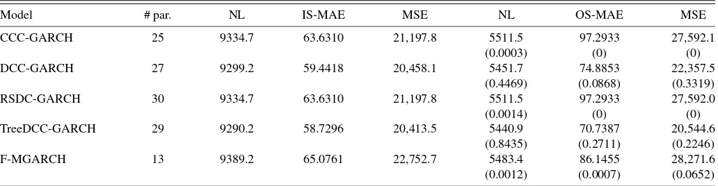
The TreeDCC model clearly has the best goodness-of-fit re-sults across all in-sample and out-of-sample measures used. The improvements in out-of-sample performance range from 1% to 25%, depending on the goodness-of-fit measure applied. Constant or piecewise-constant conditional correlation dynam-ics (like the ones implied by the CCC and RSDC models) are largely rejected by the data and lead to very inaccurate correla-tion forecasts. In contrast to the previous applicacorrela-tion to single stock returns, GARCH-type DCC effects are now crucial in or-der to improve the model’s out-of-sample forecasting power for correlations.
4.2.3 Statistical and Economic Significance of the Improve-ments. In Table5,p-values ofHansen(2005) SPA tests are reported. They show that the TreeDCC model is the only one not significantly outperformed by any other model at the 10% confidence level and for all performance criteria used.
TheEngle-DCC model yields quite good results and is not outperformed by any model at the 5% confidence level. All other models are clearly dominated at standard significance lev-els. MCS results consistently support these findings. Ten per-cent MCS using the range and the semiquadratic statistics con-sist only of the TreeDCC model for all performance criteria used. Additionally, 5% MCS include the DCC model.
Table 5. U.S. index and bond returns: Goodness-of-fit results
Model # par. NL IS-MAE MSE NL OS-MAE MSE
CCC-GARCH 25 9334.7 63.6310 21,197.8 5511.5 97.2933 27,592.1
(0.0003) (0) (0)
DCC-GARCH 27 9299.2 59.4418 20,458.1 5451.7 74.8853 22,357.5
(0.4469) (0.0868) (0.3319)
RSDC-GARCH 30 9334.7 63.6310 21,197.8 5511.5 97.2933 27,592.0
(0.0014) (0) (0)
TreeDCC-GARCH 29 9290.2 58.7296 20,413.5 5440.9 70.7387 20,544.6 (0.8435) (0.2711) (0.2246)
F-MGARCH 13 9389.2 65.0761 22,752.7 5483.4 86.1455 28,271.6
(0.0012) (0.0007) (0.0652)
NOTE: Goodness of fit of different models for a two-dimensional time series of daily (annualized) returns (in %) on the U.S. S&P500 index and the 30-year Treasury bond. Data are for the time period between January 3, 1996 and October 30, 2003, for a total of 1899 observations. The in-sample estimation period goes from the beginning of the sample to the end of 2000 (1219 observations). NL, MAE, and MSE are the multivariate versions of the standard univariate negative log-likelihood, the mean absolute error, and the mean squared error statistics. # par. reports the number of parameters estimated in the different models. For the out-of-sample performance measures,p-values of SPA tests are reported in parentheses.
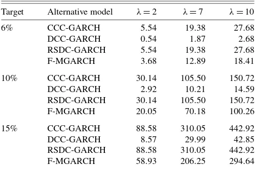
Table 6. U.S. index and bond returns: Annualized fees (in basis points)
Target Alternative model λ=2 λ=7 λ=10
6% CCC-GARCH 5.54 19.38 27.68 DCC-GARCH 0.54 1.87 2.68 RSDC-GARCH 5.54 19.38 27.68 F-MGARCH 3.68 12.89 18.41
10% CCC-GARCH 30.14 105.50 150.72 DCC-GARCH 2.92 10.21 14.59 RSDC-GARCH 30.14 105.50 150.72 F-MGARCH 20.05 70.18 100.26
15% CCC-GARCH 88.58 310.05 442.92 DCC-GARCH 8.57 29.99 42.85 RSDC-GARCH 88.58 310.05 442.92 F-MGARCH 58.93 206.25 294.64
NOTE: The table contains the annualized fees (in basis points) that a conditional mean-variance investor with absolute risk-aversion parameterλ=2, 7, and 10 will be willing to pay to perform volatility timing using the one-step-ahead conditional correlation and covariance forecasts from the TreeDCC model (benchmark model) versus those obtained using the CCC, DCC, RSDC, and the flexible MGARCH models. The portfolio weights are obtained by minimizing the one-step-ahead conditional variance forecast of a portfolio containing the U.S. S&P500 index, the 30-year U.S. Treasury bond, and the risk-free asset for a given target expected return on the portfolio. The annual risk-free rate is set to be equal to 3%. Data are for the out-of-sample time period beginning in January, 2001 and ending in October, 2003, for a total of 680 daily observations.
We conclude this section by economically quantifying the forecast improvements of our TreeDCC model relative to the competing ones. Table6presents the annualized fees (in basis points) that a conditional mean–variance investor will be ready to pay in order to forecast future variance–covariance matri-ces with the TreeDCC instead of the other models considered. The (annualized) risk-free rate is equal to 3%.
The largest economic gains arise with respect to the CCC and RSDC models: For risk aversion parameters λ≥7 and target expected returns larger than 10%, they range from ap-proximately 100 to 440 basis points per year. Sizable economic gains between 70 and 294 basis points for risk aversion pa-rameters λ≥7 and target expected returns larger than 10% also arise with respect to the flexible MGARCH model. Eco-nomic gains relative to the DCC model are small in almost all cases and never exceed 43 basis points per year. Using Diebold– Mariano-type tests we find that estimated economic gains of the TreeDCC are significant at the 1% significance level relative to the CCC and RSDC model. Estimated economic gains relative to the flexible MGARCH model are significant at the 5% signif-icance level. Improvements relative to the classical DCC model are not statistically significant. Overall, these results provide evidence that economically and statistically significant differ-ences in variance–covariance forecasts of our TreeDCC model are likely to arise with respect to the CCC, RSDC, and flexi-ble GARCH models, and less likely relative to the DCC model, which was clearly dominated by the TreeDCC model in the pre-vious empirical application.
5. CONCLUSION
We propose a new multivariate DCC-GARCH model that extends previous models by admitting multivariate thresholds in conditional volatilities and correlations. The thresholds are
modeled by a tree-structured partition of the multivariate state space and are estimated with all other model parameters. Two real data applications support the overall higher forecasting power of the TreeDCC model for return correlations, relative to Bollerslev’s CCC model, Engle’s DCC model, Pelletier’s RSDC model, and the flexible MGARCH model. We find that the conditional correlations of financial data are often charac-terized by multivariate thresholds and local GARCH-type struc-tures and that the forecast improvements of our TreeDCC model are often economically relevant. Our model can cope in a par-simonious way with such features of the data even in appli-cations with large cross sections of financial assets. An inter-esting avenue for future research is the joint empirical model-ing of the dynamic correlation of the returns of several asset classes, which are likely to exhibit rich threshold and GARCH-type effects that can be parsimoniously taken into account by our model.
APPENDIX: TESTING STATISTICAL RELEVANCE: THE MODEL CONFIDENCE SET
We formally test for differences in the forecasting power of the competing models in order to select, if possible, a best one (or a best subset of models) that significantly dominates the oth-ers in our real data application. To this end, we apply the model confidence set (MCS) method proposed byHansen, Lunde, and Nason(2003).
Without loss of generality, let us denote byDt,wkthe
differ-ences of each term in the OS-MSE statistic
Dt,wk=Ut;modelw−Ut;modelk,
t=1, . . . ,nout,w,k=1, . . . ,9,w<k,
where
nout
t=1
Ut;model=OS-MSE.
Statistics based on time averagesDwkofDt,wk allow us to
in-vestigate whether there is a systematic difference in the out-of-sample forecasting power between the different models. Tests based onDt,wk aret-type tests. In a similar way, one can
pro-ceed by using a different out-of-sample goodness-of-fit statis-tic. In our application, we compute tests based on OS-MSE, OS-MAE, and OS-NL.
The MCS is defined as the smallest set of models, which at a given confidence levelα, cannot be significantly distinguished based on forecasting power. The MCS is determined after se-quentially trimming the set of candidate models, which in our application consists of the five multivariate GARCH specifica-tions introduced earlier. At each step of such a trimming pro-cedure, the null-hypothesis of equal predictive ability (EPA)
H0:E[Dt,wk] =0,∀w,k∈M, is tested for the relevant set of
modelsMat a confidence levelα. In the first step,Mconsists
of all models under investigation. If, in the first step,H0is
re-jected, then the worst-performing model according to the rele-vant criterion is eliminated. The test procedure is then repeated for the new setM of surviving models and it is iterated
un-til the first nonrejection of the EPA hypothesis occurs. The set of resulting models is called the model confidence setMα at