Full Terms & Conditions of access and use can be found at
http://www.tandfonline.com/action/journalInformation?journalCode=ubes20
Download by: [Universitas Maritim Raja Ali Haji] Date: 11 January 2016, At: 21:58
Journal of Business & Economic Statistics
ISSN: 0735-0015 (Print) 1537-2707 (Online) Journal homepage: http://www.tandfonline.com/loi/ubes20
Examining the Distributional Effects of Military
Service on Earnings: A Test of Initial Dominance
Christopher J. Bennett & Ričardas Zitikis
To cite this article: Christopher J. Bennett & Ričardas Zitikis (2013) Examining the Distributional Effects of Military Service on Earnings: A Test of Initial Dominance, Journal of Business & Economic Statistics, 31:1, 1-15, DOI: 10.1080/07350015.2012.741053
To link to this article: http://dx.doi.org/10.1080/07350015.2012.741053
Accepted author version posted online: 06 Nov 2012.
Submit your article to this journal
Article views: 836
Examining the Distributional Effects of Military
Service on Earnings: A Test of Initial Dominance
Christopher J. BENNETT
Department of Economics, Vanderbilt University, VU Station B #351819, 2301 Vanderbilt Place, Nashville, TN 37235-1819 ([email protected])
Ri ˇcardas ZITIKIS
Department of Statistical and Actuarial Sciences, University of Western Ontario, London, Ontario N6A5B7, Canada ([email protected])
Existing empirical evidence suggests that the effects of Vietnam veteran status on earnings in the decade-and-a-half following service may be concentrated in the lower tail of the earnings distribution. Motivated by this evidence, we develop a formal statistical procedure that is specifically designed to test for lower tail dominance in the distributions of earnings. When applied to the same data as in previous studies, the test reveals that the distribution of earnings for veterans is indeed dominated by the distribution of earnings for nonveterans up to $12,600 (in 1978 dollars), thereby indicating that there was higher social welfare and lower poverty experienced by nonveterans in the decade-and-a-half following military service.
KEY WORDS: Causal effect; Crossing point; Hypothesis test; Potential outcome; Stochastic dominance; Treatment effect.
1. INTRODUCTION
Measuring and analyzing the effects of participation and treat-ment play important roles in evaluating the impact of various programs and policies, particularly in the health and social sciences (Heckman and Vytlacil 2007; Morgan and Winship
2007).
The social and economic costs of military service, for exam-ple, have drawn considerable attention from researchers and pol-icy makers, in part due to continuing military engagements and questions surrounding adequate compensation of veterans (e.g., Angrist and Chen2008; Chaudhuri and Rose2009, and refer-ences therein). Indeed, a key policy-related question is whether military service tends to reduce earnings over the life-cycle.
In this article, we focus specifically on the effect that mili-tary service in Vietnam had on subsequent earnings. Existing empirical evidence (Angrist1990; Abadie2002), for example, suggests that the effects of veteran status on earnings following service in Vietnam may have been concentrated in the lower tail of the earnings distribution. Aided with a new statistical infer-ential technique developed in this article, we examine the effect of military service on the overall distribution of earnings and on the lower tail in particular, in the decade-and-a-half following the end of war in Vietnam.
Historically, the nonrandom selection for military service has posed a significant challenge for those researching and analyzing causal effects of service. To overcome the selection problem, Angrist (1990) exploited the exogenous variation in the draft lottery to instrument for veteran status, thereby allowing for unbiased estimation of the average causal effect of service on earnings. Angrist (1990) found, for example, that white male veterans experienced roughly a 15% average loss in earnings in the early 1980s. More recently, Angrist and Chen (2008) reported that these losses in earnings dissipated over time and appear to be close to zero by the year 2000.
Abadie (2002) also exploited the variation in the draft lottery to identify the causal effect of service on earnings, focusing on the effects of Vietnam veteran status over the entire distribution of earnings. Abadie (2002) reported no statistically significant difference between the distributions of earnings for nonveterans and veterans. However, Abadie’s (2002) empirical analysis does suggest that the effects on earnings may be isolated to the lower quantiles of the earnings distributions.
Influenced by these findings, here we give a further look at the problem and investigate, roughly speaking, the range of income levels over which there are statistically significant differences in the distributions of potential earnings. A rigorous formulation of the new test, the corresponding statistical inferential theory, and subsequent empirical findings make up the main body of the present article.
To give an indication of our findings, we note at the outset that the empirical evidence points to a distribution of earnings for nonveterans that stochastically dominates the corresponding distribution of earnings for veterans for all income levels up to $12,600. This finding lends support to the aforementioned observation by Abadie (2002) concerning the isolated effects on the distribution of earnings. Furthermore, our findings suggest that, for any poverty line up to $12,600 (in 1978 dollars), there was statistically greater poverty among Vietnam veterans in the early 1980s.
The rest of the article is organized as follows. In Section2, we formulate hypotheses pertaining to the notion of “initial dominance,” explain the intuition behind these hypotheses, de-velop a large-sample theory for the corresponding test statis-tic, and illustrate the performance of the resulting test in a
© 2013American Statistical Association Journal of Business & Economic Statistics January 2013, Vol. 31, No. 1 DOI:10.1080/07350015.2012.741053
1
simulation study. In Section 3, we apply the new test to re-examine the distributional effects of military service on civilian earnings. Section4contains concluding notes. Proofs and other technicalities supporting the new test and its large-sample prop-erties are relegated to AppendicesAandB. Monte Carlo simu-lations of a more detailed nature and other supporting empirical material are given in AppendicesCandD.
2. A TEST OF INITIAL DOMINANCE
As we noted in the introduction, uncovering relationships between distributions of potential earnings for nonveterans (F) and veterans (G) is of considerable interest. For example, if F ≤Gon [0,∞), then rather powerful statements can be made concerning the comparative levels of poverty and social welfare among the groups. Specifically, if the aforementioned relation-ship between the two cumulative distribution functions (cdf’s)
F andGwere to hold, then income poverty would be greater for veterans according toanypoverty index that is symmetric and monotonically decreasing in incomes. Similarly, it is well known (see, e.g., Davidson and Duclos2000) that social welfare as measured byanysocial welfare function that is symmetric and increasing in incomes would be greater for nonveterans than for veterans.
Such interest in relationships between two cdf’s has given rise to a large literature on statistical testing procedures, and tests emerging from such constructions are usually associated with the names of Kolmogorov, Smirnov, Cram´er, Anderson, and Darling in various combinations. The use of these tests— whether two sided or one sided—presupposes that a restriction on the nature of the difference (or lack of difference) between two cdf’s must hold over their entire supports, or at least over a prespecified subset of the supports. In other words, the classical formulations impose global restrictions on the nature of the difference between the cdf’s.
In many contexts, however, it is useful to learn bothif and
wherea restriction holds, particularly when the restriction may hold only over some (unknown) subset of the supports. For example, suppose that we are interested in comparing poverty across two income distributions using the headcount ratio, which is the proportion of the population with incomes at or below a given poverty line. Because it is often difficult to reach a consen-sus on a specific value that will be used to demarcate the poverty line, an attractive procedure would be the one that would iden-tify the maximal income levelx1and hence the interval [0, x1]
over which the poverty ranking implied by the headcount rank-ing is consistent. If, for example,x1is found to be sufficiently
large by such a procedure, say so large as to constitute an upper bound for any reasonable choice of poverty line, then policy makers may reach a consensus as to the poverty ranking even without having reached a consensus on the poverty line.
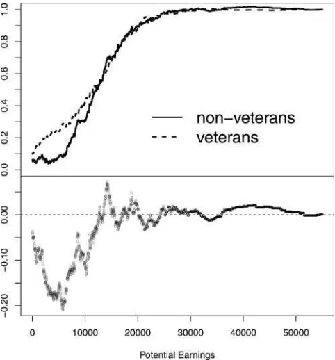
Coming now back to our underlying example of Vietnam veterans, in the context of comparing earnings distributions for the veterans and nonveterans, one distribution may not dominate another over the entire support (Figure 1) and yet the relations that hold between these two cdf’s may still be sufficient for establishing similarly powerful statements about poverty and social welfare rankings.
Figure 1. Plots of the empirical cdf’s (top panel) and their differ-ence (bottom panel) of potential earnings of nonveterans and veterans, who are compliers. (Definitions of the corresponding population cdf’s, denoted byFC
0 andF1C, will be given by Equation (3.2).
To tackle such empirical questions, in the following four sections we develop a statistical procedure that will enable us to infer the range over which a set of dominance restrictions between two cdf’s is satisfied. The procedure will allow us to (i) infer dominance with probability tending to 1 as the sample size tends to infinity whenever dominance is indeed present in the population, and (ii) consistently estimate the range over which this dominance holds. Thus, our testing procedure will help us to identify situations in whichF dominates G, and to also differentiate between situations in which this dominance holds over the entire support or only over some initial range.
2.1 Hypotheses
LetFandGbe two cdf’s, both continuous and with supports on [0,∞). Of course, we have in mind the cdf’s of potential earnings for nonveterans (F) and veterans (G), but the discussion that follows is for genericF andG, unless specifically noted otherwise.
To facilitate our discussion of the hypotheses to be tested, we first formalize the notion ofinitial dominancealong with the corresponding notion of themaximal point of initial dominance
(MPID).
Definition 2.1. We say thatF initially dominates Gup to a pointx1>0 whenF(x)≤G(x) for allx∈[0, x1) withF(x)<
G(x) for some x∈(0, x1). We call x1 the maximal point of
initial dominancewhenF initially dominates Gup tox1 and
F(x)> G(x) for allx∈(x1, x1+ǫ) for someǫ >0 sufficiently
small.
Figure 2. Illustrations of the null H0and the alternative H1. (a) Configuration in the null:Fdoes not initially dominateG. (b) Configuration in the null:Fdoes not initially dominateG. (c) Configuration in the alternative:Finitially dominatesGand the maximal point of dominancex1 is finite. (d) Configuration in the alternative:Finitially dominatesGand the maximal point of dominancex1is+∞.
Note 2.1. Definition 2.1 includes the possibility that x1=
∞, in which case the interval (x1, x1+ǫ) is empty and thus
the conditionF(x)> G(x) for allx∈(x1, x1+ǫ) is vacuously
satisfied.
Our objective in this article is (i) to infer whetherFinitially dominatesGup to some point; and (ii) in the event that initial dominance indeed holds, to produce an estimate of the MPID. Accordingly, we formulate the null and alternative hypotheses as follows:
H0:Fdoes not initially dominateG;
H1:Finitially dominatesG.
Translating H0 and H1 into formal mathematical statements,
which we shall need later in our construction of statistical tests, gives rise to:
H0:F =Gor else there existsǫ >0 such thatF(x)≥G(x)
for allx∈[0, ǫ) withF(x)> G(x) for somex ∈(0, ǫ); H1: There existx1∈(0,∞] and ǫ >0, such that F(x)≤
G(x) for allx∈[0, x1) with some x∗∈(0, x1) such that
F(x∗)< G(x∗), andF(x)> G(x) for allx∈(x1, x1+ǫ).
The null hypothesis H0 includes all possible configurations
of F and Gfor which F does not initially dominate G. This
occurs, for example, whenever the configurations of FandG
are such thatFstarts out aboveG. Two such configurations are illustrated in panels (a) and (b) ofFigure 2. First, in panel (a), the distribution F starts out aboveGand then crosses below, while in panel (b),Fonce again starts out aboveGbut in this case it remains there over the entire support.
Also, Fdoes not initially dominate Gwhen equality holds between the distributions so that
F(x)=G(x) for all x ∈[0,∞). (2.1)
Consequently, the statement of the null hypothesis H0 also
in-cludes this configuration, which is at the “boundary” between the null H0 and the alternative H1. We will see below that this
“boundary” case plays a special role when calculating critical values of the new test.
The alternative hypothesis H1 includes all possible
config-urations of F and Gfor which F initially dominatesG. The parameterx1, which appears under the statement of the
alterna-tive, corresponds to the MPID as defined above in Definition 2.1. WhenFinitially dominatesG, the MPIDx1, which is generally
unknown, may be anywhere to the right of zero. For example, whenFinitially dominatesGandx1is finite, then it must be the
case that the cdf’s cross atx1(see, e.g., panel (c) ofFigure 2).
Alternatively, whenFinitially dominatesGandx1= ∞, then
initial dominance holds over the entire supports and we have
FdominatingGin the classical sense of stochastic dominance. This latter situation is depicted in panel (d) ofFigure 2.
The alternative of initial dominance is of particular interest in our investigation of earnings and poverty, because finding initial dominance would, for example, imply that a broad class of poverty measures agree on a poverty ranking (Davidson and Duclos 2000). As a concrete example, consider the popular Foster, Greer, and Thorbecke (1984) poverty measure defined by
πα,x(F)=E[gα(X;x)1{X≤x}], (2.2)
where X with the cdfF is income,x ≥0 is the poverty line, g(y;x)=(x−y)/x is the normalized income shortfall, and α≥0 is an indicator of “poverty aversion.” IfFinitially domi-natesG, then for every level of poverty aversion, the FGT mea-sure recordsπα,x(F)≤πα,x(G) for all poverty lines 0≤x ≤x1
with strict inequality holding for some poverty lines 0≤x≤x1.
Initial dominance thus guarantees that every FGT poverty mea-sure records poverty to be at least as great inGfor any poverty line in the interval (0, x1) and strictly greater inG for some
poverty lines in the interval (0, x1).
2.2 Parametric Reformulation
To construct a test for H0 against H1, we employ a
one-dimensional parameterθsuch that the hypotheses can be refor-mulated as follows:
H0 :θ=0
H1 :θ >0. (2.3)
To defineθ, we first introduce an auxiliary function:
H(y)= y
0
(F(x)−G(x))+dx,
wherez+=0 whenz≤0 andz+ =zwhenz≥0. The function H(y) is nonnegative, takes on the value 0 at y=0, is non-decreasing, and has a finite limiting value H(∞) as long as both F andG have finite first moments. Next, we define the generalized inverse ofH(y)
H−1(t)=inf{y ≥0 :H(y)≥t},
which is a nondecreasing and left-continuous function that may have jumps (e.g., a jump att =0). We then use this generalized inverse to define the point
x1=lim
t↓0H
−1(t). (2.4)
The pointx1will play a pivotal role in our subsequent
consider-ations because whenFinitially dominatesG, thenx1as defined
in Equation (2.4) is equivalent to the MPID as introduced in Definition 2.1. Of course, the parameter x1 in Equation (2.4)
remains well defined whenFdoes not initially dominateG(i.e., under H0); however, it is no longer interpretable as an MPID in
this case.
With this pointx1, we defineθby the formula
θ=
x1
0
(G(x)−F(x))+dx.
(Note that the integrand in the definition ofθ is the positive part ofG(x)−F(x), unlike the integrand in the definition of H(y), which is the positive part ofF(x)−G(x).) Under the null H0, we haveθ=0 irrespectively of whetherx1is finite or
infinite. Under the alternative H1, the parameterθ is (strictly)
positive becauseF(x) dips strictly below G(x) at least at one pointx ∈(0, x1). These are the properties of θ postulated in
Equation (2.3).
2.3 Statistics and Their Large Sample Properties
We next construct an estimator for θ. To begin with, let X1, . . . , Xn be independent random variables fromF, and let Y1, . . . , Ymbe independent random variables fromG. These
ran-dom variables are also assumed to be independent between the samples. (We refer to Linton, Song, and Whang (2010) for tech-niques designed to deal with correlated samples.) Denote the corresponding empirical cdf’s byFn andGm, and then define
an estimator ofH(y) by the formula
Hm,n(y)=
y
0
(Fn(x)−Gm(x))+dx.
The corresponding generalized inverse is
Hm,n−1(t)=inf{y ≥0 :Hm,n(y)≥t}.
We next define an estimatorxm,n ≡xm,n(δm,n) of the pointx1
by the formula
xm,n=Hm,n−1(δm,n),
whereδm,n >0 is a “tuning” parameter such that
δm,n↓0 and
nm
n+mδm,n→ ∞ (2.5)
when min{m, n} → ∞. Hence, this tuning parameter cannot be overly small, nor too large, and thus in a sense resembles the “bandwidth” choice in the classical kernel density estimator. We shall elaborate on practical choices ofδm,n below, particularly
when discussing simulation results and analyzing the veteran data. We note that, throughout this article, we letmandntend to infinity in such a way that
m
n+m→η∈(0,∞) (2.6)
meaning that the two sample sizes are “comparable,” which is a standard assumption when dealing with two samples.
The estimatorxm,n of x1<∞ as formulated above is
de-signed to detect the first point after which the sample analogue of F (i.e., Fn) crosses above the sample analogue of G(i.e., Gm). Ideally, this estimator will consistently estimate the
pa-rameterx1 <∞, which is equal to the MPID under H1, and
otherwisex1(finite or infinite) is well-defined though no longer
interpretable as an MPID under H0. When working with these
sample analogues, we thus allow for some “wiggle room” in the sense that Fn is said to cross above Gn at xm,n only if
xm,n
0 (Fn(z)−Gm(z))+dzexceeds the threshold parameterδm,n.
The reason why we cannot setδm,nto zero is because the
func-tionFn−Gmis “rough” (think here very appropriately of the
Brownian bridge) even when the population cdf’sFandGare identical on [0,∞).
The choice ofδm,n clearly influences how sensitive the
esti-mator ofx1is to regions for whichFnis observed to cross above Gm. Takingδm,nto be small means thatδm,nwill, roughly
speak-ing, pick off the first point in the sample at whichFncrosses
aboveGm as the estimate ofx1. On the other hand, whenδm,n
is chosen to be large, thenFnwill be allowed to cross above Gm for some time before the threshold is reached andxm,n is
declared. We shall elaborate on this point in the next section. With the estimator xm,n of x1 in hand, we next define an
estimatorθm,nofθby
θm,n=
xm,n
0
(Gm(x)−Fn(x))+dx.
The following six theorems make up our large-sample asymp-totic theory for the estimatorsxm,n andθm,n. We begin by
in-vestigating the consistency of the estimatorxm,nunder both the
null and alternative hypotheses.
Theorem 2.1. WhenF =G on [0,∞) or, more generally, whenF ≤G on [0,∞), thenx1= ∞andxm,n→P ∞when min{m, n} → ∞.
Theorem 2.2. Under the alternative H1, and also under the
null H0with the exception of the case whenF ≤Gon [0,∞)
(which is covered by Theorem 2.1), we have that the pointx1is
finite andxm,n→Px1when min{m, n} → ∞.
We next investigate the asymptotic behavior of the suitably scaled version of the estimatorθm,n, namely
m,n=
whereBdenotes the standard Brownian bridge.
Theorem 2.3 has assumed a little bit more than two finite moments ofFandG, but this is a negligible assumption given the underlying problem.
Theorem 2.4. Under the null H0, with the exception of the
caseF =Gon [0,∞) that has been covered by Theorem 2.3,
where the pointx1, calculated using Equation (2.4), is finite.
Hence, the limiting integral in Equation (2.8) is smaller than that in Equation (2.7), which proves the least-favorable nature of the critical values calculated under the (null) sub-hypothesis F =Gon [0,∞).
The remaining two theorems shed further light on the behav-ior ofm,n. The first theorem deals with the case whenx1 is
finite.
Theorem 2.5. Under the alternative H1, and assuming that the
pointx1is finite, we have thatm,n →P∞when min{m, n} → ∞.
The final theorem of this section deals with the case when the pointx1is infinite.
Theorem 2.6. Suppose that X andY have 2+κ finite mo-ments for some κ >0, no matter how small. When F ≤G but F =G on the entire [0,∞), and thus x1 = ∞, then
m,n →P∞when min{m, n} → ∞.
The proofs of the above theorems are given in AppendixB. The next section outlines the practical implementation of the above-developed statistical inferential theory.
2.4 Practical Implementation
In view of the above theory, we retain the null H0 when the
value ofm,nis small and reject when it is large, with “small”
and “large” determined by a critical value calculated using the following bootstrap algorithm (cf., e.g., Section 3.7.2 of van der Vaart and Wellner1996; Barrett and Donald2003; Horvath, Kokoszka, and Zitikis2006):
Algorithm 2.1. The following steps produce the bootstrap crit-ical valuecm,n(α):
1. Form the pooled distribution Lm,n(x)=(mGm(x)+ nFn(x))/(m+n).
2. Generate mutually independent iid samplesX∗
1, . . . , X∗nand
wherexm,n∗ is the bootstrap analogue ofxm,nbased on
boot-strap samples generated in Step 2.
4. Repeat Steps 2 and 3Btimes and record{∗m,n,b(x∗m,n,b),1≤ b≤B}.
5. The nominal α level critical value, which we denote by cm,n(α), is then computed as the (1−α) quantile of the
dis-tribution of bootstrap estimates from Step 4:
cm,n(α)=inf
With the critical valuecm,n(α), the decision rule at the nominal
levelαis to reject H0in favor of H1, and thus infer that there is
“initial dominance” over the interval [0, xm,n), whenever
m,n> cm,n(α).
For more details on the practical implementation of this boot-strap procedure, we refer to Barrett and Donald (2003); in our simulation studies, we have also closely followed this article.
The above bootstrap procedure is designed to estimate the critical value in the least favorable case (i.e.,F =Gon [0,∞)) under the null. We note that it is also possible to implement a bootstrap procedure that uses the estimatorxm,n in place of x∗
m,n in Step 3 of Algorithm 2.1. However, implementing this
modified bootstrap procedure would require us to incorporate
Andrews and Shi’s (2010) infinitesimal uniformity factor, or a similar method used by Donald and Hsu (2010), to well control the size of the test since both the test statistic and the boot-strap critical value based on∗
m,n(xm,n) would converge to zero
wheneverx1=0. Because the additional complexity (e.g., the
introduction of an additional tuning parameter) would invari-ably cause us to stray from the main contribution of this article, we do not adopt such a procedure in the present article.
Theorem 2.7 shows that the bootstrap procedure outlined in Algorithm 2.1 yields asymptotically valid tests that are also consistent.
Theorem 2.7. Suppose that X andY have 2+κ finite mo-ments for someκ >0, no matter how small. Then we have
lim
m,nP[m,n> cm,n(α)|H0]≤α, (2.10)
and
lim
m,nP[m,n > cm,n(α)|H1]=1, (2.11)
where the limits are taken with respect to the sample sizesm
andntending to infinity in a way such that conditions (2.5) and (2.6) are satisfied.
We next illustrate the performance of the proposed testing procedure, with more detailed simulation results exhibiting
both the power and good finite sample control of the size relegated to Appendix C. For this, we generate independent log-normal samples X1, . . . , Xn and Y1, . . . , Ym according
to Xi =exp(σ1Z1i+µ1) and Yi =exp(σ2Z2i+µ2), where
the Zki’s are independent standard normal random variables.
Various choices of the parameter-pairs (µi, σi) are explored in
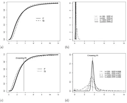
the simulation study, and they are specified in the legends of the left-hand panels ofFigure 3.
The figure illustrates the performance of the test under two different scenarios:
Panels (a) and (b):Fstarts out aboveGand crosses below at some later point, which is a null H0 configuration; see
panel (a) ofFigure 2.
Panels (c) and (d):Flies belowGup to a point and crosses above thereafter, which is an alternative H1configuration;
see panel (c) ofFigure 2.
Hence, panels (a) and (b) are in the null H0. Panels (c) and
(d), on the other hand, reflect a configuration ofFandGin the alternative H1. The two left-hand panels (a) and (c) illustrate
the relationships between the cdf’s under consideration, and the right-hand panels (b) and (d) illustrate the densities ofxm,nfor
different sample sizes, along with the corresponding empirical rejection probabilities (EPRs). Recall that the pointxm,nis
com-puted prior to testing, irrespective of whether we have H0or H1.
Figure 3. Monte Carlo illustrations based on parent cdf’s (left-hand panels) with the corresponding density plots (right-hand panels) ofxm,n
estimates, along with ERPs at the 5% nominal level. (a) A null H0configuration withF=LN(0.7,0.8) andG=LN(0.85,0.6). (b) Density plots ofxm,nestimates. (c) An alternative H1configuration withF=LN(0.85,0.6) andG=LN(0.7,0.8). (d) Density plots ofxm,nestimates.
But the point xm,n is referred to as the estimated MPID only
under the alternative H1, which defines “initial dominance.”
We have conducted 1000 bootstrap resamples in each of the 5000 Monte Carlo replications, setting δm,n=κ((m+ n)/(mn))1/2−ǫwithκ
=10−6andǫ
=0.01. (For more details on the tuning parameterδm,n, its robustness with respect to choices
ofκandǫ, we refer to Section3.3and AppendixD.) The follow-ing information can be gleaned from the plots. First, in panels (a) and (b), which correspond to the null configuration in which
Fis initially dominated byG, we see from the concentration of the density plots about the origin that the initial dominance ofG
overFis detected in virtually all of the Monte Carlo trials. More importantly, we have not detected a single instance in which the null would be erroneously rejected.
When there is a region of initial dominance as in panel (c) of
Figure 3, it is desirable that our test procedure have appreciable power to detect the presence of dominance and to also return a reliable estimate of the region over which initial dominance holds. Panel (d) ofFigure 3reports that the test has considerable power to detect the region of initial dominance even in samples consisting of only 100 observations. As expected, the density plots show that in such small samples there is a great deal of variation in the estimated MPID about the true value, and we also see that the densities of the estimated MPID become increasingly concentrated around the true value as the sample sizes are increased.
3. VIETNAM VETERAN DATA REEXAMINED
Here we apply the new test to reexamine distributional ef-fects of Vietnam veteran status on labor earnings. Abadie (2002) showed that the potential distributions for veterans and nonvet-erans can be estimated for the subpopulation of compliers, and he used Kolmogorov-Smirnov type tests to empirically examine whether the earnings distribution of nonveterans stochastically dominates that of veterans. Using the same dataset, we shall see below that the new test allows us to make statistically significant statements concerning the effect of veteran status on poverty.
3.1 The Potential-Outcomes Model
Let Z be a binary instrument, taking on the values 0 (not draft eligible) and 1 (draft eligible) with some positive probabil-ities, and letD(0) andD(1) denote the values of the treatment indicator Dthat would be obtained given Z=0 and Z=1, respectively. BothD(0) andD(1) are random, taking on the val-ues 0 (do not serve in the military) and 1 (serve in the military) with some positive probabilities. The binary nature of both the instrument and the treatment variables gives rise to four possible types of individuals in the population:
• Compliers whenD(0)=0 andD(1)=1 • Always-takers whenD(0)=1 andD(1)=1 • Never-takers whenD(0)=0 andD(1)=0 • Defiers whenD(0)=1 andD(1)=0
Because our interest centers on the causal effect of military service on earnings, letY(1) denote the potential incomes for individuals if they served (D=1) andY(0) denote the potential
incomes for the same individuals had they not served (D=0). In practice, the analyst observes only the realized outcomes
Y =Y(1)D+Y(0)(1−D), (3.1)
where D=D(1)Z+D(0)(1−Z). Within this framework of potential incomes, the distributional effect of military service in the general population is captured by the difference between the cdf’s of Y(0) andY(1). However, neither of the two cdf’s is identified because, among other things, the data are (i) un-informative aboutY(0) in the subpopulation of always-takers, and also (ii) uninformative aboutY(1) for the subpopulation of never-takers. Because of this identification problem, it is com-mon in the treatment effects literature to focus the analysis on the subpopulation of compliers. In the context of examining for distributional treatment effects, this amounts to comparing the conditional cdf’sF0C andF1Cdefined by
FkC(y)=P[Y(k)≤y|D(0)=0, D(1)=1], (3.2)
where, naturally, we assume thatP[D(0)=0, D(1)=1]>0, which means that compliers are present in the general popula-tion. We shall elaborate on the latter assumption at the end of the next section.
3.2 An Underlying Theory
When comparing FC
0 and F1C, we are particularly
inter-ested in establishing whether (cf. the alternative H1 of
“ini-tial dominance”) there exists a level of income y1 such that
F0C(y)≤F1C(y) for all y∈[0, y1) with the inequality being
strict over some subset of [0, y1). Inferring the existence of such
an income level would allow us to make statistically significant statements concerning poverty and social welfare orderings of the two distributions.
We note in this regard that any member of the earlier noted FGT (Foster, Greer, and Thorbecke1984) class of poverty mea-sures would indicate that poverty is at least as great or greater among those in the subpopulation of compliers who served in the military for any poverty line in the interval [0, y1). Similarly, for
anyy∗ ∈[0, y
1) and every monotonic utilitarian social welfare
function when applied to the censored distributions generated by replacing incomes abovey∗ byy∗ itself would rank the
so-cial welfare of nonveterans equal to or higher than veterans. We refer to, for example, Foster and Shorrocks (1988) for details.
The task of testing for an initial region of dominance (com-pared to the alternative H1) among the subpopulation of
compli-ers can be simplified by the fact that we do not actually need to estimate the two complier cdf’s but rather examine the sign of the difference between these cdf’s. Specifically, we shall show in the next theorem that the relationship of initial dominance, or lack thereof, betweenFC
0 andF1C can be investigated in terms
of two other cdf’s, namelyF0andF1defined by
Fk(y)=P[Y ≤y|Z=k]. (3.3)
Theorem 3.1. Assume that, forz=0 and also forz=1, the triplet{Y(1), Y(0), D(z)}is independent ofZ. If there are no
defiers, then for everyywe have that F0(y)−F1(y)=F0C(y)−F
C
1(y)
P[D(0)=0, D(1)=1]. (3.4)
Hence, in particular, F0(y)≤F1(y) if and only if F0C(y)≤
F1C(y).
The proof of Theorem 3.1 is relegated to AppendixA. Hence, by Theorem 3.1, we have that the differenceF0−F1is
proportional to the differenceF0C−F1C, and the proportionality coefficient is the population proportionP[D(0)=0, D(1)=1] of compliers.
We conclude this section with a note that even though we explicitly make only Condition 1(i) by Imbens and Angrist (1994) in Theorem 3.1, our earlier made assump-tion P[D(0)=0, D(1)=1]>0 of the presence of compli-ers in the general population together with the assumption of no defiers in Theorem 3.1 imply part (ii) of Condition 1 by Imbens and Angrist (1994); the latter condition means that
P[D(1)=1]>P[D(0)=1]. The proof that the condition holds under the assumptions of the present article consists of just a few lines:
P[D(1)=1]=P[D(1)=1, D(0)=0]
+P[D(1)=1, D(0)=1],
P[D(0)=1]=P[D(0)=1, D(1)=0]
+P[D(0)=1, D(1)=1].
The right-most probabilities in both equations are the same, and the absence of defiers makes the middle probability in the second equation vanish. Hence, subtracting the first equation from the second one, we obtain the equation
P[D(1)=1]−P[D(0)=1]=P[D(0)=0, D(1)=1],
which proves the fact that, throughout the present article, we work under the entire Condition 1 by Imbens and Angrist (1994). Hence, this setup is equivalent to that by Abadie (2002) (see Assumption 2.1 therein).
3.3 The Veteran Data and Test Results
In our empirical analysis, we use the CPS extract (Angrist
2011) that was especially prepared for Angrist and Krueger (1992). This same dataset was also used by Abadie (2002). As described in the latter article, the data consist of 11,637 white men, born in 1950–1953, from the March Current Population Surveys of 1979 and 1981–1985. For each individual in the sample, annual labor earnings (in 1978 dollars), Vietnam veteran status, and an indicator of draft eligibility based on the Vietnam-era draft lottery outcome are provided. Following Angrist (1990) and Abadie (2002), we use draft eligibility as an instrument for veteran status. The construction of the draft eligibility variable is described in Appendix C of the literature by Abadie (2002). Additionally, a discussion of the validity of draft eligibility as an instrument for veteran status may be found in the paper by Angrist (2002).
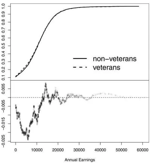
The empirical counterparts ofF0andF1are simpler to work
with, given the dataset that we are exploring, and are thus
adopted in our test of initial dominance.Figure 4displays the empirical distributionsF0,n0andF1,n1. (Compare this figure with Figure 1, where the latter depicts the empirical distributionsF0C,n
0
andFC
1,n1.)
Applying the test for initial dominance to this data with the conservative choice of parameter values κ =10−6 and
ǫ=10−2, for example, yields an estimated MPID x
1 of
ap-proximately $12,600 with a corresponding bootstrapp-value of 0.063. With a significance levelα >0.063, therefore, we would reject H0 and conclude that F0C initially dominates F
C
1 up to
$12,600, thereby implying that Vietnam veterans experienced poverty at least as great as nonveterans based on any poverty line up to $12,600. We note that this finding is also robust over a reasonably wide set of choices for the tuning parameterδn0,n1.
Indeed, an examination of the empirical results (see Appendix D) over the grid of δn0,n1’s computed from combinations of ǫ∈ {10−j,1
≤j ≤5}andκ ∈ {10−j,1
≤j ≤6}reveals that the crossing point estimates never fall below $12,600 and are all associated withp-values no larger than 0.073.
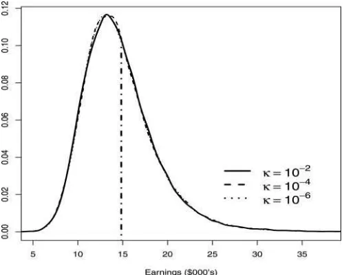
The figure $12,600 is of course just an estimate of the popu-lation MPID, and it is therefore only natural when interpreting the above statement to wonder about the statistical uncertainty attached to this figure. To address the question of statistical un-certainty we would ideally report the standard error attached to this estimate, or provide a confidence interval. However, pro-ducing such figures gives rise to a number of difficult problems (see Note B.1 in AppendixBfor more details) that are beyond the scope of the current article. For example, because the MPID is interpretable only under the alternative and is thus reported only upon rejection of the null hypothesis, determining the sam-pling distribution of the MPID estimator first requires fixing a
Figure 4. Plots of the empirical cdf’s (top panel) and their difference (bottom panel) of actual earnings of nondraft-eligible and draft-eligible, who may or may not be compliers. (Definitions of the corresponding population cdf’sF0andF1are in Equation (3.3).
Figure 5. Density plots corresponding to estimates of the MPID. The plots are generated usingδn0,n1=κ((n0+n1)/(n0n1))
0.49 based
on samples generated from log-normal distributions calibrated to the data. The vertical dashed line marks the location of the MPID for the calibrated distributions.
configuration under the alternative and then computing the dis-tribution conditional on rejection. Second, the variability of the MPID estimator will hinge critically on the rate of departure of
FfromGto the right of the MPIDx1, measuring which would
require imposing conditions on the densities as well as on higher derivatives of the cdf’sFandG. (See Note B.1 in AppendixB
for a further discussion on these points.)
In the absence of a formal theory, however, we have con-ducted a small simulation exercise to give a general sense of the statistical uncertainty that might be attached to a point esti-mate of the MPID such as that reported above. This simulation exercise involves drawing samples of sizen0 andn1from
log-normal distributions that are calibrated to match the first and second moments ofF0,n0andF1,n1.Figure 5plots the densities
arising from the use ofδn0,n1=κ/((n0+n1)/(n0n1))
0.49withκ
set to 10−2, 10−4, and 10−6(it suffices to examine the variation
inκ only because the sample sizes are fixed). The plots reveal that the densities are rather insensitive to variation inκ. Also, the plots show the mode of the density in each case to be around $12,000, whereas the true MPID is around $14,800 for our cho-sen log-normal populations. Lastly, the standard errors in each case are found to be around $4,000.
4. CONCLUDING NOTES
In many practical situations, it is unlikely that dominance relations hold over the entire support of the distributions under consideration. However, a number of results in the literature (e.g., Foster and Shorrocks1988) demonstrates that even when a dominance relation holds only on a subset of the support, we may still obtain powerful orderings in terms of poverty or social welfare. With this in mind, in this article we have developed a statistical test that enables one to infer whether there exists an initial region of stochastic dominance, and also to infer the range over which the dominance relation holds. Notably, the test
can also be used to establish dominance over the entire support. This occurs whenever dominance is indicated by our procedure
andthere is an absence of crossing in-sample.
Our work on this statistical inference problem has been in-spired by existing empirical evidence (Angrist 1990; Abadie
2002) suggesting that the effects of Vietnam veteran status on earnings are concentrated in the lower tail of the earnings dis-tribution. In particular, the inferential procedure developed in the present article was specifically designed to test for the ex-istence of lower tail dominance in the distributions of earnings. When applied to the same data used in previous studies, our test indicates that the distribution of earnings for veterans (i.e.,
G) is initially dominated by the distribution of earnings for nonveterans (i.e.,F) up to $12,600 in 1978 dollars, thereby sug-gesting that there was higher social welfare and lower poverty experienced by nonveterans in the decade-and-a-half following military service.
A number of interesting problems remain for future work. Among them would be to develop a theory for the standard errors attached to the MPID estimates, and establishing asymptotically valid confidence intervals for this parameter of interest. Though interesting, we anticipate these problems to be highly technically demanding.
APPENDIX A: PROOF OF THEOREM 3.1
We first rewrite the underlying probabilities as expectations of the corresponding indicator random variables and in this way have the equation
F0(y)−F1(y)=E[1{Y ≤y}|Z =0]−E[1{Y ≤y}|Z=1].
Next we write each indicator 1{Y ≤y}as the sum of 1{Y ≤y}D and 1{Y ≤y}(1−D), and using the additivity of expectations, we then obtain the equation
F0(y)−F1(y)=E[1{Y ≤y}D|Z =0]
−E[1{Y ≤y}D|Z=1]
+E[1{Y ≤y}(1−D)|Z=0]
−E[1{Y ≤y}(1−D)|Z=1]. (A.1)
Upon recalling definition (3.1) of the random variable Y, we have from Equation (A.1) that
F0(y)−F1(y)
=E[1{Y(1)D(0)+Y(0)(1−D(0))≤y}D(0)|Z=0] −E[1{Y(1)D(1)+Y(0)(1−D(1))≤y}D(1)|Z=1]
E[1{Y(1)D(0)+Y(0)(1−D(0))≤y}(1−D(0))|Z=0] −E[1{Y(1)D(1)+Y(0)(1−D(1))≤y}(1−D(1))|Z=1].
(A.2)
Now we drop the conditioning from every expectation on the right-hand side of equation (A.2) because, by our assumption, for z=0 and also forz=1, the triplet {Y(1), Y(0), D(z)}is independent ofZ. In summary, we have that
F0(y)−F1(y)=A(y)+B(y), (A.3)
where
We proceed by splitting each of the expectations making up the definitions ofA(y) andB(y) into four parts, according to the subdivision of the sample space into four groups as mentioned at the beginning of Section3.1. For example, forA(y) we have the equation (with expectations converted back into probabilities)
A(y)=P[Y(1)≤y|D(0)=1, D(1)=1]
The first and fourth probabilities cancel out. Since we assume that there are no defiers, which means thatP[D(0)=1, D(1)= 0]=0, we finally arrive at the equation
A(y)= −F1C(y)P[D(0)=0, D(1)=1].
Analogously, we obtain that
B(y)=F0C(y)P[D(0)=0, D(1)=1].
Plugging in the above expressions forA(y) and B(y) on the right-hand side of Equation (A.3), we obtain Equation (3.4). This concludes the proof of Theorem 3.1.
APPENDIX B: ASYMPTOTIC TECHNICALITIES
There are two goals that we accomplish in this section. First, we need to prove the six theorems formulated in Section2.3, as they comprise the large-sample statistical inferential theory for the test of “initial dominance.” Second, since the asymptotic critical values depend on the unknown underlying distributions, we also need to justify the bootstrap procedure formulated in Section2.4.
We start with the inferential theory. Throughout, we use the notation
m,n(x)=(Fn(x)−F(x))−(Gm(x)−G(x)).
Proof of Theorem 2.1.SinceF ≤Gon [0,∞) by assumption, the functionHis equal to 0 on the entire half-line [0,∞), and thus x1= ∞. We shall next show that the estimator xm,n≡ xm,n(δm,n) converges to∞in probability, which means that, for
everyM >0,
In view of assumption (2.5), statement (B.1) holds provided that
nm
n+mHm,n(M)=OP(1),
which is a consequence of
This concludes the proof of statement (B.1) as well as that of
Theorem 2.1.
Proof of Theorem 2.2.Keeping in mind that the cdf’sFand
Gare not identical throughout this proof, and irrespectively of whether we are dealing with the null H0 or the alternative H1,
we always havex1∈[0,∞) andǫ >0 such that
We first establish statement (B.2):
PHm,n−1(δm,n)> x1+γ
The right-hand side converges to 0 becauseδm,n→0,
x1+min{γ ,ǫ}
This concludes the proof of statement (B.2).
To prove statement (B.3), we write:
hand side of bound (B.4) converges to 0 in probability because of assumption (2.5) and the fact that
nm
n+m
x1−γ
0 |
m,n(z)|dz=OP(1).
This concludes the proof of statement (B.3) as well as that of
Theorem 2.2.
Note B.1. We cannot theoretically derive confidence intervals that would asymptotically maintain the prespecified level, and the reason for this is two-fold: (i) the tuning parameter δm,n
influences the normalizing constant needed for establishing the limiting distribution of the appropriately scaled and normalized estimatorxm,nin a way similar to the influence of the bandwidth
in the kernel density estimator, and (ii) the limiting distribution depends in a crucial way on the rate of departure ofFfromG
to the right of the pointx1, which imposes conditions on the
densities as well as on higher derivatives ofFandGthat we do not want to highlight in the article. On the other hand, a kind of a conservative confidence interval is already provided by the consistency statement of Theorem 2.2. Indeed, the established fact thatxm,nconverges in probability tox1means that, for every
γ >0 andα∈(0,1],
P[|xm,n−x1|> γ]≤α (B.5)
for all sufficiently largen. This is proved in Theorem 2.2. Ideally, we would like to haveγdependent on the sample sizesmandn
and converging to 0 when the sample sizes get larger, in such a way that the probability in (B.5) would asymptotically be equal toα. Because of both the aforementioned reasons, we cannot achieve such aγ but we see from the proof of Theorem 2.2 that we can easily find someγ ≡γm,n→0 such that it would still
satisfy statement (B.5). Indeed, we just need to chooseγm,n→0
such that the integral
x1+γm,n
x1
(F(z)−G(z))+dz
would converge to 0 slower thanδm,n to assure the validity of
statement (A.2). This can certainly been done, but the choice of such aδm,nwould depend on the slope of the functionz→
(F(z)−G(z))+ immediately to the right of the pointx1. This
clarifies point (2) above.
Proof of Theorem 2.3.We begin by noting that the integral in statement (2.7) is well defined and finite (almost surely), because the cdfFhas 2+κfinite moments for someκ >0, no matter how small. By Markov’s inequality, this follows if we verify that the expectation of the integral is finite, and we do this next:
The integral on the right-hand side is finite because of the afore-mentioned moment assumption onF, which implies the inte-grability of the function √1−F(x) over the entire half-line (0,∞).
We shall now start proving statement (2.7). From Theorem 2.1 we have that when F =G on [0,∞), then x1= ∞ and
Choose any (small)ν >0. We have that
∞ finite moments for someκ >0. Furthermore, sinceF =Gon [0,∞), we have that
This concludes the proof of Theorem 2.3.
Proof of Theorem 2.4. From the definition of the pointx1
given by Equation (2.4), we see that under the null H0, the point
x1is the largestxsuch thatF(x)=G(x). Note that the pointx1
is finite under the assumption of the theorem, because if it were infinite, then we would be under the subnull hypothesisF =G on [0,∞), which is excluded. Hence,x1<∞, and in this case
we also have thatF(x)> G(x) at least for somexto the right ofx1. Furthermore, by Theorem 2.2 we have thatxm,n→P x1.
With the above information, we proceed as follows:
Hence, we have expressedm,nas a linear combination of four
quantities. The second one converges to 0 becausexm,n →Px1
and
nm
n+mz∈sup[0,∞)|
m,n(z)| =OP(1), (B.8)
by the classical Kolmogorov-Smirnov theorem. The fourth quantity converges to 0 because of the same reasons, plus the fact that G(z)< F(z) for all z∈(x1, xm,n) and for all
suffi-ciently largemandnso thatxm,nwould be sufficiently close to x1with as large a probability as desired. Hence,
m,n =
where B1 and B2 are two independent standard Brown-ian bridges. But under the null H0 we have F(x)=G(x)
for all x∈[0, x1). Hence, the processes {√ηB1(F(z))+
√
1−ηB2(G(z)), z∈[0, x1)} and {B(F(z)), z∈[0, x1)}
co-incide in distribution. This concludes the proof of
Theorem 2.4.
Proof of Theorem 2.5. By Theorem 2.2, we have thatx1 is
finite andxm,n →Px1. Next we write the bounds
sufficiently smallτ >0, we have that
x1−τ
of Theorem 2.5 is finished.
Proof of Theorem 2.6.We start with a bound:
m,n=
which holds for every pair (F, G). Due to the assumption thatX
andYhave 2+κ finite moments for someκ >0, we have that
Sincexm,n→P ∞, the first integral on the right-hand side of bound (B.13) tends to ∞ in probability provided that, for a sufficiently largeM <∞,
M so the right-continuity of the cdf’s implies that M
0 (G(z)−
F(z))+dz >0 for all sufficiently largeM <∞. This concludes
the proof of Theorem 2.6.
Having thus established the six theorems upon which our statistical inferential theory hinges, we next justify the use of the aforementioned bootstrap procedure. This requires us to prove Theorem 2.7.
Proof of Theorem 2.7. We need to prove statements (2.10) and (2.11). Let us assume temporarily that
∗m,n(xm,n∗ )⇒P ∞
0
(√ηB1(F(z))+1−ηB2(G(z)))+dz,
(B.16)
where ⇒P denotes conditional weak convergence in probabil-ity. Under this assumption, statement (2.10) is an immediate consequence of Theorem 1 by Beran (1984) because
lim
m,nP[m,n> cm,n(α)|H0]≤limm,nP[m,n> cm,n(α)|F =G],
(B.17)
and
Moreover, when statement (B.16) holds, then so does (2.11). This is because m,n→P∞ under H1 (c.f. Theorem 2.5),
whereascm,n=OP(1) as a consequence of (B.16).
We are therefore left to prove statement (B.16). Toward this objective, letFn∗ andG∗m denote the empirical cdf’s based on independent random samples of sizen andmdrawn from the pooled set of observationsZ= {X1, . . . , Xn, Y1, . . . , Ym}. The-orem 3.7.6 by van der Vaart and Wellner (1996) gives
nm
This result will be used in the proof of statement (B.16), which involves several steps. First, we examine the behavior of the bootstrap estimate of
Second, we establish the asymptotic distribution of the corre-sponding bootstrap statistic∗
m,n.
To begin, letP∗ denote the probability measure induced by
the bootstrap conditional onZ. Our first objective is to show that, for allM >0,
P∗[xm,n∗ (δm,n)≥M]→1 (B.21)
in probability. Using the fact that the boundx∗
m,n(δm,n)≥Mis
it suffices to show that
P∗
in probability. However, the assumption nm
n+mδm,n→ ∞
to-with the latter being a direct consequence of Equation (B.19), imply the convergence in Equation (B.23) and, hence, give the desired result.
We next examine the limiting behavior of the bootstrap statistic
Due to Equation (B.19), the second term on the right-hand side of Equation (B.25) satisfies
∞
/2−νdzis finite for any sufficiently small
ν >0. Consequently, statement (B.16) holds. This completes
the proof of Theorem 2.7.
APPENDIX C: SIMULATION DETAILS
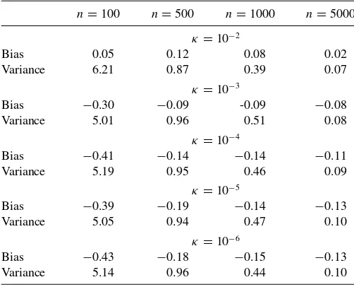
Table C1. Estimated bias and variance ofx1estimators based on
δm,n=κ((m+n)/(mn))1/2−ǫwithn
=mandǫ=0.1. The estimates correspond to different choices ofκand are computed using 5000
Monte Carlo replications withB=1000 bootstrap samples
n=100 n=500 n=1000 n=5000
κ=10−2
Bias 0.05 0.12 0.08 0.02
Variance 6.21 0.87 0.39 0.07
κ=10−3
Bias −0.30 −0.09 -0.09 −0.08
Variance 5.01 0.96 0.51 0.08
κ=10−4
Bias −0.41 −0.14 −0.14 −0.11
Variance 5.19 0.95 0.46 0.09
κ=10−5
Bias −0.39 −0.19 −0.14 −0.13
Variance 5.05 0.94 0.47 0.10
κ=10−6
Bias −0.43 −0.18 −0.15 −0.13
Variance 5.14 0.96 0.44 0.10
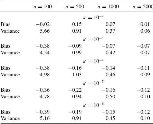
Table C2. Estimated bias and variance ofx1estimators based on
δm,n=κ((m+n)/(mn))1/2−ǫwithn
=mandǫ=0.01. The estimates correspond to different choices ofκand are computed from
5000 Monte Carlo replications withB=1000 bootstrap samples
n=100 n=500 n=1000 n=5000
κ=10−2
Bias −0.02 0.15 0.07 0.01
Variance 5.66 0.91 0.37 0.06
κ=10−3
Bias −0.38 −0.09 −0.07 −0.07
Variance 4.54 0.99 0.42 0.07
κ=10−4
Bias −0.38 −0.16 −0.14 −0.11
Variance 4.98 1.03 0.46 0.09
κ=10−5
Bias −0.36 −0.22 −0.16 −0.12
Variance 4.78 0.94 0.50 0.10
κ=10−6
Bias −0.39 −0.19 −0.15 −0.12
Variance 5.16 0.91 0.45 0.10
Table C3. Estimated size of dominance tests at the 5% nominal level whenF=G=LN(0.85,0.6) based onδm,n=κ((m+n)/(mn))1/2−ǫ
withn=m. Empirical rejection probabilities are reported for various values ofκandǫ, and are computed from 5000 Monte Carlo
replications withB=1000 bootstrap samples
κ n=100 n=500 n=1000 n=5000
ǫ=0.1
10−2 0.041 0.042 0.047 0.052
10−3 0.044 0.041 0.044 0.049
10−4 0.040 0.043 0.043 0.041
10−5 0.042 0.039 0.042 0.042
10−6 0.039 0.041 0.043 0.041
ǫ=0.01
10−2 0.043 0.042 0.043 0.050
10−3 0.042 0.044 0.043 0.043
10−4 0.043 0.042 0.042 0.043
10−5 0.042 0.040 0.042 0.041
10−6 0.041 0.041 0.042 0.042
Table C4. Estimated power of dominance tests at the 5% nominal level againstF=LN(0.85,0.6) andG=LN(0.7,0.8) based on
δm,n=κ((m+n)/(mn))1/2−ǫwithn
=m. Empirical rejection probabilities are reported for various values ofκandǫ, and are computed from 5000 Monte Carlo replications withB=1000
bootstrap samples
κ n=100 n=500 n=1000 n=5000
ǫ=0.1
10−2 0.398 0.978 1.000 1.000
10−3 0.603 0.979 0.993 1.000
10−4 0.634 0.981 0.988 0.998
10−5 0.664 0.981 0.989 0.997
10−6 0.658 0.979 0.989 0.997
ǫ=0.01
10−2 0.397 0.984 1.000 1.000
10−3 0.603 0.979 0.993 1.000
10−4 0.657 0.979 0.989 0.998
10−5 0.661 0.977 0.987 0.997
10−6 0.662 0.980 0.989 0.997
APPENDIX D: SENSITIVITY OF THE EMPIRICAL RESULTS TO THE CHOICE OF TUNING PARAMETER
Table D1. Estimated crossing points and correspondingp-values based on 5000 bootstrap replications with the tuning parameter
δm,n=κ((m+n)/(mn))1/2−ǫfor various values ofκandǫ
κ
ǫ 10−1 10−2 10−3 10−4 10−5 10−6
10−1 $12,654 $12,606 $12,604 $12,604 $12,604 $12,604
0.064 0.073 0.070 0.072 0.073 0.069
10−2 $12,639 $12,605 $12,604 $12,604 $12,604 $12,604
0.066 0.070 0.068 0.070 0.071 0.063
10−3 $12,638 $12,605 $12,604 $12,604 $12,604 $12,604
0.077 0.062 0.067 0.068 0.072 0.074
10−4 $12,638 $12,605 $12,604 $12,604 $12,604 $12,604
0.076 0.073 0.072 0.067 0.076 0.065
10−5 $12,638 $12,605 $12,604 $12,604 $12,604 $12,604
0.079 0.063 0.071 0.077 0.073 0.066
ACKNOWLEDGMENTS
We are grateful to Keisuke Hirano, an anonymous associate editor, and two anonymous reviewers for critical remarks, sug-gestions, and advice that resulted in a substantial revision of the article. The second author also thanks the Department of Economics at Vanderbilt University for hospitality during his stay at the university while working on the project, and he also gratefully acknowledges the financial support for his visit pro-vided by the Grey fund. The research was also supported by the Natural Sciences and Engineering Research Council (NSERC) of Canada.
[Received December 2011. Revised August 2012.]
REFERENCES
Abadie, A. (2002), “Bootstrap Tests for Distributional Treatment Effects in Instrumental Variable Models,”Journal of the American Statistical Associ-ation, 97, 284–292. [1,7,8,9]
Andrews, D. W., and Shi, X. (2010),Inference Based on Conditional Moment Inequalities, Cowles Foundation Discussion Papers 1761, New Haven, CT: Cowles Foundation for Research in Economics, Yale University. [6] Angrist, J. D. (1990), “Lifetime Earnings and the Vietnam Era Draft Lottery:
Evidence From Social Security Administrative Records,”American Eco-nomic Review, 80, 313–336. [1,8,9]
——— (2011), “CPS Extract,” Data File [online]. Available at http://econ-www.mit.edu/faculty/angrist/data1/data/angkru95[accessed May 5, 2011]. Angrist, J. D., and Chen, S. (2008),Long-Term Economic Consequences of Vietnam-Era Conscription: Schooling, Experience and Earnings, IZA Dis-cussion Papers 3628, Bonn: Institute for the Study of Labor (IZA). [1]
Angrist, J. D., and Krueger, A. B. (1992),Estimating the Payoff to School-ing UsSchool-ing the Vietnam-Era Draft Lottery, NBER Working Papers 4067, Cambridge, MA: National Bureau of Economic Research. [8]
Barrett, G. F., and Donald, S. G. (2003), “Consistent Tests for Stochastic Dom-inance,”Econometrica, 71, 71–104. [5]
Beran, R. J. (1984), “Bootstrap Methods in Statistics,” Jahresbericht der Deutschen Mathematiker-Vereinigung, 86, 14–30. [12]
Chaudhuri, S., and Rose, E. (2009),Estimating the Veteran Effect With Endoge-nous Schooling When Instruments are Potentially Weak, IZA Discussion Papers 4203, Bonn: Institute for the Study of Labor (IZA). [1]
Davidson, R., and Duclos, J.-Y. (2000), “Statistical Inference for Stochastic Dominance and for the Measurement of Poverty and Inequality,” Econo-metrica, 68, 1435–1464. [2,4]
Donald, S., and Hsu, Y.-C. (2010), “Improving the Power of Tests of Stochastic Dominance,” Working paper.
Foster, J., Greer, J., and Thorbecke, E. (1984), “A Class of Decomposable Poverty Measures,”Econometrica, 52, 761–766. [4,7]
Foster, J. E., and Shorrocks, A. F. (1988), “Poverty Orderings and Welfare Dominance,”Social Choice and Welfare, 5, 179–198. [7,9]
Heckman, J. J., and Vytlacil, E. (2007), “Econometric Evaluation of Social Programs, Part I: Causal Models, Structural Models and Econometric Pol-icy Evaluation,” inHandbook of Econometrics(1st ed., Vol. 6B), eds. J. Heckman and E. Leamer, Amsterdam: Elsevier, chap. 70. [1]
Horvath, L., Kokoszka, P., and Zitikis, R. (2006), “Testing for Stochastic Dom-inance Using the Weighted McFadden-Type Statistic,”Journal of Econo-metrics, 133, 191–205. [5]
Imbens, G. W., and Angrist, J. D. (1994), “Identification and Estima-tion of Local Average Treatment Effects,” Econometrica, 62, 467– 475. [8]
Linton, O., Song, K., and Whang, Y.-J. (2010), “An Improved Bootstrap Test of Stochastic Dominance,” Journal of Econometrics, 154, 186– 202. [4]
Morgan, S., and Winship, C. (2007),Counterfactuals and Causal Inference: Methods and Principles for Social Research, New York: Cambridge Uni-versity Press. [1]
van der Vaart, A., and Wellner, J. (1996),Weak Convergence and Empirical Processes: With Applications to Statistics, New York: Springer. [5,13]