Full Terms & Conditions of access and use can be found at
http://www.tandfonline.com/action/journalInformation?journalCode=ubes20
Download by: [Universitas Maritim Raja Ali Haji] Date: 12 January 2016, At: 01:07
Journal of Business & Economic Statistics
ISSN: 0735-0015 (Print) 1537-2707 (Online) Journal homepage: http://www.tandfonline.com/loi/ubes20
IT and Beyond: The Contribution of Heterogeneous
Capital to Productivity
Daniel J. Wilson
To cite this article: Daniel J. Wilson (2009) IT and Beyond: The Contribution of Heterogeneous Capital to Productivity, Journal of Business & Economic Statistics, 27:1, 52-70, DOI: 10.1198/ jbes.2009.0005
To link to this article: http://dx.doi.org/10.1198/jbes.2009.0005
Published online: 01 Jan 2012.
Submit your article to this journal
Article views: 70
View related articles
IT and Beyond: The Contribution of
Heterogeneous Capital
to Productivity
Daniel J. W
ILSONFederal Reserve Bank of San Francisco (Daniel.Wilson@sf.frb.org)
This article explores the relationship between capital composition and productivity using a unique, detailed dataset on firm investment in the United States in the late 1990s. I develop a methodology for estimating the separate effects of multiple capital types in a production function framework. I back out the implied marginal products of each capital type and compare these with rental price data. I find that although most capital types earned normal returns, information and communications technology capital goods had marginal products substantially above their rental prices. The article also provides evidence of complementarities and substitutabilities among capital types and between capital types and labor.
KEY WORDS: Capital heterogeneity; Information and communications technology; Investment;
Production function estimation.
1. INTRODUCTION
There has been a tremendous amount of public interest and debate during the past several years on how information and communication technologies (ICT) affect productivity. A number of studies have found that ICT investment is associated with higher labor productivity even after controlling for ICT’s contribution to capital deepening. This leads one to ask: Is ICT special? That is, does investment in ICT equipment have a greater impact on productivity than investment in other capital goods? Are there other specific capital goods that contribute to productivity in disproportion to their share of capital? More generally, does the mix of capital affect productivity? This article seeks to answer these questions.
Understanding how ICT interacts with other capital goods in production is of fundamental importance to understanding the nature of the production function. It is also particularly relevant for understanding the sources of the rapid increase in aggregate total factor productivity (TFP) during the past decade, a period in which the mix of physical capital in the economy has changed dramatically. Beyond the specific issue of the ICT– productivity link, previous research has not examined em-pirically the relationship between the entire capital mix and productivity. This article is able to do so by making use of the micro level data from a unique, highly detailed survey of U.S. businesses: the 1998 Annual Capital Expenditures Survey (ACES).
The special focus on ICT up until now is understandable given its increasingly vital role in business and personal activity. However, there are several reasons to expand our attention beyond the productivity impact of ICT to the impact of other capital goods as well, and, in fact, to expand our attention to the impact of the capital mix more generally. First, computers, software, and communications equipment are not purchased in isolation. They are often purchased in conjunction with other capital goods to build a system of capital to accomplish productivity enhancements. Thus, even if one’s interest is only in the productivity impact of ICT, one must account for its correlation with other specific capital goods that have their own impact on productivity. Second, policymakers
considering incentives such as investment tax credits and accelerated depreciation allowances aimed at increasing pro-ductivity need to know which capital asset types should be targeted. (See House and Shapiro [2008] for a discussion of the effects of the temporary accelerated depreciation allowances enacted in the United States in 2002 and 2003, which differ-entially favored long-lived capital types.) For this purpose, one must know the productivity impacts of every type of capital. Third, nearly all microlevel production studies are forced, given data limitations, to assume a single, homogenous capital stock (two at most). In reality, capital is clearly heterogeneous. The potential measurement error arising from this assumption has long been recognized (Solow 1955–1956; Fisher 1965; Jorgenson and Griliches 1967), but the data necessary to address this concern has not previously been available at the micro level.
The goal of this article is to begin to fill in the gap in our understanding of the relationship between capital mix and productivity. The article offers four main contributions. First, I construct a unique, new firm-level dataset, combining data on asset-specific investment with data on output and factor inputs (among other variables), that allows one to investigate the contribution of heterogenous capital to output and productivity. Specifically, I match firm observations from the Census Bureau’s recent ACES of 1998, which contains investment broken out across a wide range of separate capital types, to the Compustat research file and its data on output and factor inputs for 1998 and subsequent years for publicly traded firms. As is frequently the case with large-scale survey data, the ACES reflects a tradeoff between data richness (i.e., how much detail is requested of respondents) and the frequency of collection. Thus, it is important to acknowledge at the outset that the tremendous richness of these data, in terms of providing quite disaggregate investment for a large cross-section of firms, comes at the cost of having no time dimension. This precludes
52
2009 American Statistical Association Journal of Business & Economic Statistics January 2009, Vol. 27, No. 1 DOI 10.1198/jbes.2009.0005
the use of panel data econometric techniques for addressing endogeneity concerns, although I use a number of other ap-proaches to address these concerns.
The second contribution of the article is to develop a succinct methodology for modeling the separate effects of a large number of capital types in a production function framework. I show that, under relatively mild conditions, these effects can be estimated via linear regression analysis using data on invest-ment mix along with total capital stock and other factor inputs. The third contribution is to use this methodology, combined with recently developed techniques for accounting for unob-served productivity, to identify the effects of different types of capital on output and to back out the implied marginal products of different types of capital. The baseline regression results clearly indicate that investment in computers, communications equipment, software, and offices is positively associated with both current and subsequent years’ output, conditional on total capital and labor. I perform a number of exercises to determine the primary direction of causality explaining these correlations. I find these results are robust to including either a 1-year lead of the firm’s Solow residual or a polynomial of investment, cap-ital, and age (a` la Olley and Pakes 1996) in the regressions, both of which are techniques for directly controlling for unobserved productivity. However, including a proxy for organizational capital wipes out the offices–productivity association while leaving the association for the ICT capital types, suggesting ICT capital has a causal effect on output even after controlling for the effects of total capital and labor.
I then back out the marginal products of different capital types implied by the regression results and compare them with data on rental prices provided by the U.S. Bureau of Labor Statistics (BLS). For the most part, the implied marginal products are strikingly similar to these rental price estimates, as would be predicted by standard neoclassical theory. However, for a few key types like computers, communications equip-ment, and software, the implied marginal products are found to be substantially higher than the official rental prices. The implied excess returns to ICT capital suggest differential adjustment costs among capital types, unobserved comple-mentary coinvestments with ICT capital, or systematic expec-tational errors by firms regarding the relative marginal products of different capital goods.
This article’s fourth contribution is to test for production complementarities and substitutabilities among capital goods, and between different types of capital and labor. I find strong evidence of such complementarities and substitutabilities. In particular, using any reasonable division of types into ‘‘tech’’ and ‘‘low-‘‘tech’’ categories, the data indicate that high-tech capital goods tend to be complementary with low-high-tech capital goods and substitutable with other high-tech capital. Not only does this result have interesting implications for productivity, it also is a rejection of the assumption that capital goods are perfectly substitutable, an assumption researchers are often forced to make in the empirical productivity liter-ature. I also find complementarities and substitutabilities between certain capital types and labor. For instance, software is found to be especially labor-saving, whereas general-purpose machinery and trucks are especially labor-augmenting. Given the well-documented shifts in aggregate capital composition in
the United States during the past decade or so, this result may have implications for trends in labor demand and relative wages.
The organization of this article is as follows: Section 2 dis-cusses the previous literature investigating the relationship between ICT investment, or the capital mix more broadly, and productivity. Section 3 derives the empirical model that I estimate and discusses the econometric issues that arise. The data that I use are summarized in Section 4. Section 5 describes the main results, where capital type investment shares are not interacted with each other or with labor. Section 6 describes the results of adding these interactions to investigate complemen-tarities and substitutabilities among capital types, and between capital types and labor. Section 7 concludes.
2. BACKGROUND
As mentioned at the start of the article, up to this point, the literature on the productivity impact of disaggregate investment has focused almost exclusively on computers and communi-cations equipment (and mostly just computers). (An exception is the study by Caselli and Wilson 2004, who used country-level data on capital imports to explore the determinants of capital composition and its effects on labor productivity.) The macroeconomic literature typically has relied on growth-accounting exercises to explore the issue (Oliner and Sichel 1994; Gordon 2000; Jorgenson and Stiroh 2000; Oliner and Sichel 2000), whereas microeconomic studies generally have relied on firm- or establishment-level production function estimation, with ICT capital as a separate production input in addition to labor and non-ICT capital (Brynjolfsson and Hitt 1996; Lehr and Lichtenberg 1999; Greenan and Mairesse 2000; Brynjolfsson and Hitt 2003; Gilchrist, Gurbaxani, and Town 2003; and Hempell 2005).
During the 1980s and the first half of the 1990s, most studies found little or no evidence of an economically important contribution of information technology (IT) or ICT on pro-ductivity or propro-ductivity growth (Griliches and Siegel 1992; Oliner and Sichel 1994; Berndt and Morrison 1995). More recently, a consensus appears to be forming that IT and ICT investment are positively associated with conventionally measured TFP, although the magnitude, direction of causality, and timing of this association is still very much under debate. Oliner and Sichel (2000) used growth-accounting techniques to identify the contribution, within a standard neoclassical pro-duction framework, of IT capital to aggregate productivity growth. They found that the use and production of IT equip-ment together account for two thirds of the acceleration in productivity growth that occurred between the first half and the second half of the 1990s (see Jorgenson and Stiroh 2000 for similar results).
On the micro side, Brynjolfsson and Hitt (1995, 1996) estimate that the returns to IT spending are substantially higher than those to non-IT spending. Greenan and Mairesse (2000) find evidence that computer use has a positive impact on pro-ductivity at the firm level using data on the French manu-facturing and services sectors. However, they cannot reject the hypothesis that the computer’s contribution to productivity is the same as the contribution of other capital. Gilchrist et al.
(2003) use a modified version of the Arellano and Bond (1991) generalized method of moments estimator to estimate the elasticity of the IT capital stock via both a production function and a multifactor productivity (MFP) framework. They find that IT’s elasticity in the production function is about equal to its cost share and is not significant in the MFP regression, both consistent with normal returns within the neoclassical model. However, they also find that personal computers have an impact on productivity above and beyond their contribution to the IT stock, at least for the durable good sector. Brynjolfsson and Hitt (2003) estimate the elasticity of computers using both short- and long-difference regressions. They find that com-puters’ elasticity is consistent with their cost share in the short differences; but, consistent with Gilchrist et al. (2003), the long-difference results suggest excess returns, because the computers’ elasticity is significantly higher than computers’ cost share.
Although these and other studies in the productivity liter-ature to date have generally focused exclusively on computers (and, to a lesser extent, communications equipment), the investment literature has explored the implications of capital heterogeneity more broadly for adjustment costs (Hayashi and Inoue 1991; Chirinko 1993) and tax policy (Cummins, Hassett, and Hubbard 1994; Goolsbee 2004; House and Shapiro 2008). Most relevant to this article, Cummins and Dey (1998) estimate a structural model in which heterogeneous capital goods are allowed to affect production and adjustment technologies dif-ferentially, and find important effects of imperfect substitut-ability. Their capital stock data, however, are only broken down into two groups: equipment and structures.
3. EMPIRICAL MODEL
The focus of this article is on the relationship between het-erogeneous capital services and labor productivity at the firm level. The goal of this section is to derive an empirical, firm-level production function specification incorporating het-erogeneous capital services based on standard neoclassical production theory. This theory, dating back to Solow (1955– 1956), contends that the services of heterogeneous capital goods can be expressed as a single aggregate quantity, X ¼
g(X0,X1,. . .,XN), if the marginal rate of substitution between any two capital goods is independent of the quantity of labor. The production function for a firm (or the economy as a whole) can then be treated as a function of labor and this single capital aggregate.
Unfortunately, the appropriate aggregator function g() is unknown. Fisher (1965) demonstrated that if different types (or vintages) of capital embody different levels of quality (i.e., they have different marginal products), then there is an additional necessary and sufficient condition for the existence of a single capital aggregate: The heterogeneous quality must be expres-sible in homogenous constant-quality units (this is the well-known ‘‘better¼more’’ assumption. This condition along with the weak separability with labor are equivalent to requiring that different capital types be perfect substitutes after they have been measured in constant-quality units. A firm’s total capital services then can be expressed as a sum of individual capital services, weighting each by its relative marginal product.
It is important to distinguish this exercise of measuring the
quantity of total capital services with the far more common exercise, done in growth-accounting studies, of measuring the
changein total capital services. The goal in growth accounting is to decompose the change in output (for a firm, industry, or economy) into the change in inputs, including capital services, and the change in TFP. As Jorgenson and Griliches (1967) and others have shown, when one is only seeking to measure the change in total capital services and not the actual quantity, one need not make the restrictive assumptions discussed earlier. (In particular, perfect substitutability between different capital goods is not required.) Rather, a Divisia index (e.g., Tornqvist) of total capital services can be constructed from observed changes in the quantities of subaggregate capital services. Of course, as an index number, this index provides no information about the actual level of capital services, only its current level relative to past levels. Hence, it is of no use in measuring the true quantity of capital services entering a firm’s production function, which is what one needs to estimate production parameters using cross-firm regression analysis. It is worth noting, though, that Jorgenson and Griliches (1967) (and sub-sequent growth-accounting studies like that conducted by Jorgenson and Stiroh 2000) do in fact use an arithmetic sum, as I do here for total capital services, to measure thelevelof the capital services forsubaggregatesof capital goods. And, as I do here, they point out that the key to aggregating goods within a subaggregate group is that the units of each good be converted to a common base by using their relative marginal products.
Assuming the Solow-Fisher conditions hold, a firmihas total capital services, Xi, equal to the weighted sum of individual
capital services:Xi¼ PN
j¼0 1þuj
Xij, wherejindexes capital types and 1þuj
are weights that sum to N, the number of capital types. If I make the further assumption that each indi-vidual capital service is proportional to the firm’s stock of capital of that type (i.e., utilization rates do not vary across types), thenXij¼bKijandXi¼b
PN
j¼0 1þuj
Kij, whereKijis
the stock of capital of type j. Thus, total capital services is proportional to a weighted sum of individual capital stocks. The role of the weights, 1þuj, is to convert whatever unitsKijis
measured in into constant-quality units that can be compared across types. By settingu0¼0, we choose the units of capital
type 0 as the basis of measurement for all goods. As shown later, the weights represent the marginal products of each capital type relative to the marginal product of the base type. In the data used in this article, the units of capital type 0 are dollars (book value). Hence, the weights in the capital services summation can be thought of as converting the dollar value of each capital type into its equivalent dollar value in terms of the base capital type, using their relative marginal products for the conversion.
For example, suppose a firm has a stock of computers and a stock of tractors with equal market values. As we know from Hall and Jorgenson’s (1967) work on the user cost of capital, even though the market values of these two capital stocks are equal, the flow of capital services they provide, and hence their marginal products, may be very different. For instance, a higher marginal product of computers may be offset by a higher rate of depreciation, leaving the return to computers equal to the return to tractors. If the marginal product of tractors were our base of measurement, then an appropriate measure of the total flow of
capital services for this firm would be proportional to (with factor of proportionality b) the stock of tractors plus the product of the stock of computers and the ratio of the marginal product of computers to the marginal product of tractors.
Now let us define the production function for output. I assume a standard Cobb-Douglas production function in terms of capital services (Xi) and labor (Li) with a Hicks-neutral
stock, measured in current dollars andKiis the total book value
of capital. It is straightforward to verify that 1þuj
is the ratio of the marginal product of typejcapital to that of the base type:
Thus,ujrepresents the percentage difference between capital
type j’s marginal product and the marginal product of the numeraire capital type. In the standard neoclassical model, optimizing firms choose the quantity of each input such that its marginal product is equal to its implicit rental price (user cost), in which case the input is said to be earning normal returns. The ratio between the marginal products of different capital stocks is then equal to the ratio of their user costs (see Jorgenson 1963). Thus, the standard neoclassical model would predict that 1þuj¼ cj=c0, where cj and c0 are the user costs for
type-jand type-0 capital, respectively.
There are a number of possible reasons, however, that 1þuj¼ cj=c0might not hold. First, there could be
adjust-ment costs and/or learning-by-doing processes that differ-entially affect capital goods. For instance, Cummins and Dey (1998) estimated that adjustment costs for equipment capital are significantly different (lower, in general) than for structures capital, suggesting that differences likely exist among types within these broad categories as well. In addition, a number of studies have analyzed recent and historical episodes wherein productivity was adversely affected in the short run by learning costs involved with the introduction of either new types of capital goods to existing production processes or preexisting capital goods to new applications (e.g., see David’s 1990 study of computers in the 1960s through 1980s and the electric dynamo at the turn of the past century). Second, there may be unobserved organizational coinvestments, such as new work-place practices and management systems, associated with particular capital goods (e.g., see Bresnahan and Greenstein 1996; Black and Lynch 2001; Brynjolfsson et al. 2002; Bresnahan, Hitt, and Yang 2002; Bartel et al. 2007; and Bloom, Sadun, and Van Reenen 2007 regarding links between recent changes in management techniques and IT capital). Third, as a result of uncertainty regarding the rate of return on capital investments,
there could be systematic expectational errors by firms that may be more severe for certain capital goods, particularly new and/or rapidly changing capital goods. Of course, these three possible causes of nonnormal returns are not mutually exclu-sive. For example, errors in expected productivity gains from particular capital investments may be related to unexpectedly high learning/adjustment costs or to unanticipated needs for additional investments in organizational capital.
The principal focus of the empirical analyses in this article is on obtaining consistent estimates of the set of uj’s (i.e., the
relative marginal products of heterogeneous capital types). To estimate theuj’s via linear regression, the production
func-tion must first be linearized. If P
j¼1ujðKij=KiÞ 0 (recall P
j¼1uj¼0), then, to an approximation, the production func-tion in logs becomes
subscripts. This equation forms the basis for the primary regression specification I use to investigate the association between individual capital types and output conditional on total capital and labor.
Note that any approximation error introduced here is likely to result in a negative bias in ordinary least squares (OLS) estimation of theuj’s. For simplicity, consider the case when
there is only one capital type (j ¼ 1) in addition to the numeraire type. As u1K1/K diverges from zero, the
approx-imation error, log(1þu1K1/K)u1K1/K, which is an omitted
variable in the estimation, will become increasingly negative. So if the trueu1is nonzero, then the omitted variable will be
more negative for firms with larger shares of investment in type 1. Hence, there will be a negative bias on the estimator ofu1. In
particular, notice that any findings of excess returns that one obtains are likely to be underestimates whereas findings of below-normal returns may be overstated.
As noted in the introduction, an important limitation of the 1998 ACES data are that they contain disaggregateinvestment, but not disaggregatecapital stocks. Hence, capital sharesKijt/
Kit are unobserved. Investment shares Iijt/Iit, however, are
observed, and with the proper data, capital shares can be approximated from investment shares. From the standard capital accumulation equations,Iijt¼DKij,tþ1þdjKijtandIit¼
growth rates of capital type j and total capital, respectively. Unfortunately, these growth rates of capital are unobserved in the data. If the growth rates are small (relative to the depreci-ation rates), as would be expected in a steady state, the first term in the previous product is approximately equal to the ratio of total depreciation to type-jdepreciation. To the extent that firms deviate from balanced growth, the bias (on the estimator of uj) caused by omitting the difference between the capital
share and the investment share in a regression is likely to be negative. The reasoning goes as follows: Type-specific
investment is likely to be lumpy over time, so a high (condi-tional on industry and other regressors), type-jinvestment share this period generally signals a low beginning-of-period type-j
capital stock share. Thus, the partial correlation betweenIij/Ii
and the omitted variable (Kij/Ki Iij/Ii) is negative, which
implies a negative bias on the estimator of the investment share’s coefficient (auj). In particular, significantly positive
estimates of auj, such as those obtained later for computers,
software, and communications equipment, cannot be explained by this omitted variable bias.
Earlier, I showed that uj represents the relative marginal
product of type-j capital (less one). Using investment shares in lieu of capital shares in our regressions thus changes the interpretation of uj from Fj=F0
. Likewise, I showed earlier that the neoclassical prior (based on firms choosing factor quantities until marginal products equal rental prices) for this parameter is cj=c01. Using investment shares, this prior becomes
cj=c01
d=dj
. In Section 5.2, I back out the marginal products implied by the estimated^uj’s and compare them to the widely used user cost estimates generated by BLS.
Returning to the specifications discussed earlier, the shift variable,ait, is an unobserved variable that is likely to vary by
firm and may possibly be correlated with the other regressors. To formalize this possibility let us rewriteaitas
ait¼mitþyit: ð5Þ
The first term, mit, is the component of productivity that is
known, or ‘‘transmitted,’’ to the firm when it makes its variable input decisions, but it is unobserved by the econometrician. This term encompasses both time-invariant and time-varying productivity factors (known to the firm). The second term,
yit, is a productivity innovation that isex anteunknown even to
the firm. It is orthogonal to all factor inputs including the capital mix. The concern with estimating equation (3) via OLS is that transmitted productivity, mit, may be correlated with
the firm’s input decisions, including the capital composition decision, leading the OLS estimator of our parameters to be biased.
One often can control at least for the time-invariant aspects ofmit(i.e., firm fixed effects) through panel data methods (e.g.,
first-differencing). In this article, however, I have only a single cross-section of data, for 1998, on Kjit/Kit (although data for
subsequent years are available for the variablesYit,Kit, andLit).
Because of this limitation of the data, my identification strategy is to focus on the cross-sectional estimation and include potential proxies or correlates of both the time-varying and time-invariant aspects ofmit.
At a minimum, one can attempt to account formitwith a set
of control variables:
I refer to this equation as the ‘‘baseline regression.’’ The first set of control variables are meant to capture permanent firm
characteristics. These consist of three-digit SIC-level industry dummy variables, location (state) dummies, and a five-category indicator of firm size (employment); this size variable is described in Appendix A. The state (of headquarters) dummy is included because a number of studies have found that loca-tion has an important effect on firm performance; this effect can be due, for example, to networks/technological spillovers or density (Audretsch and Feldman 1996; Ciccone and Hall 1996; Ellison and Glaeser 1999). I also include a dummy variable indicating whether the firm had an investment spike (investment equaling 20% or more of the beginning-of-year book value of capital, which is a common spike definition in the literature (Doms and Dunne 1998)). The investment spike dummy is included because firms with a spike may incur high short-run adjustment costs resulting in lower output, ceteris paribus. Conversely, the spike may reflect the firm’s response to a positive productivity shock (similar to how investment is argued to reflect unobserved productivity shocks in Olley and Pakes 1996). Either way, it should be included in the re-gression, because investment spikes may consist dispropor-tionately of certain capital goods (as found in Wilson 2008), thus excluding the spike variable could bias the coefficients on the investment shares of those capital goods.
Because it is unlikely the transmitted productivity term,mit,
will be fully captured by these control variables alone, I investigate three alternative approaches that build on the baseline regression presented earlier. The first approach fol-lows the Olley and Pakes (1996) technique. Olley and Pakes (1996) show that under certain conditions—notably perfect competition and the exogeneity ofmitwith respect to the firm’s
variable input decisions—current investment will be a mono-tonic function ofmit, the capital stock, and age. The
monoto-nicity of this unknown function implies that mit will be a
function of investment, capital, and age. They suggest proxying for this unknown function using a kernel estimator or a poly-nomial. I follow this approach using a third-order polynomial (including interaction terms). In our particular context, the validity of the Olley-Pakes approach requires one additional condition: The transmitted productivity shock should affect total investment demand, but not the composition of invest-ment. One can get some sense of the validity of this condition by comparing the estimated coefficients on the capital-type investment shares from a regression in which the investment shares are lagged 1 year (i.e., all variables are 1999 values except the 1998 investment shares), and hence are pre-determined, to those from a regression with all contempora-neous (1998) values. I do so in Section 5 and find that the estimated coefficients are quite similar.
The second approach is to include a measure of one-year-ahead Solow residual as an additional regressor (relative to the baseline regression). The Solow residual is defined as srdit ¼
ln(Yit) sitK ln(Kit) sitL ln(Lit), where sitK and sitL are the
observed factor shares of capital and labor, respectively (see Appendix A for how these shares were measured). Note that even though capital shares are only observed in our data for 1998, the components of the Solow residual (which come from Compustat) are observed in other years as well. From equations (3) (substituting for capital shares with investment shares) and (5), one obtains
lnðYi;99Þ ¼mi;99þyi;99þalnðKi;99Þ þblnðLi;99Þ
Note that the unobserved, transmitted productivity term,mi,99,
can be decomposed into a time-invariant fixed effect,fi, and a
year-specific component,vi,99. Furthermore, recall thatyi,99is
an iid productivity innovation (uncorrelated withyi,98). Thus,
one can see that adding srdi,99as an additional regressor to the
baseline (1998) regression should control for the fixed effect,fi,
as well as the transmitted productivity shockvi,98to the extent
thatvi,tfollows an AR(1) process (because vi,99 ¼rvi,98 þ
ei,99, whereei,99is iid). Note, however, that there may be serious multicollinearity from having both the 1998 investment shares and srdi,99, which is affected by the 1999 investment shares, as
regressors. This multicollinearity will bias upward the standard errors on the estimates ofauj. Although they reduce precision,
this bias in the standard errors has the virtue that it reduces the likelihood of a false finding of statistical significance on the investment share coefficients. Therefore, this regression pro-vides a useful check on the consistency of the baseline results. Lev and Radhakrishnan (2005), among others, have argued that firm-level organizational capital can be proxied by a firm’s selling, general, and administrative (SGA) expenses. SGA (by Compustat’s definition) includes advertising/marketing expenses, amortization of research and development costs, cost of engineering services, leasing costs, and freight costs. These types of costs can be thought of as investments in the firm’s knowledge base, brand reputation, and distribution capacity, which collectively comprise its ‘‘organizational capital.’’ Both the time-invariant and time-varying components of the unob-served, transmitted productivity term (mit) are likely to be
strongly correlated with organizational capital, and hence SGA. Therefore, our fourth approach is to include (log) SGA as an additional regressor in equation (6) to control for unob-served, transmitted productivity.
In all regressions, I measure output using firm sales deflated by a three-digit industry price deflator corresponding to the firm’s predominant industry. I opt to use a gross output (sales) concept instead of real value-added due to the well-known problem that properly measuring the latter requires a separate materials costs deflator, which is not available. As is common in the literature (Bahk and Gort 1993; Burnside Eichenbaum, and Rebelo 1995; Basu 1996; Basu and Fernald 1995; Lev and Radhakrishnan 2005), I exclude intermediate expenses (mate-rials) in the Cobb-Douglas portion of the production function and thus the estimating equation. This exclusion amounts to assuming that the gross output (GOit) production function is
Leontief (weakly separable) in value added (Yit) and materials (Mit):
GOit¼minðYit;MitÞ:
Because this production function implies ln(GOit) ¼ ln(Yit),
one can estimate equation (3) by simply replacing ln(Yit),
which is not observed in the data without substantial mea-surement error, with ln(GOit), which is observed in the data.
Another option is to assume that the gross output production function is Cobb-Douglas in capital, labor,and materials and then include ln(Mit) as an additional regressor. There are a
couple of reasons, however, why omitting materials is pref-erable. First, including materials would limit our sample size considerably because Compustat does not contain intermediate expenses for a number of companies. More important, inter-mediate expenses in Compustat are subject to a serious mea-surement error that is likely correlated with capital composition. A large share of certain types of investment, particularly soft-ware, communications equipment, and instruments, may be expensed by companies rather than capitalized and therefore reported as intermediate expenses rather than capital invest-ment. Given that the unobserved, omitted measurement error corresponding to observed ln(Mit) is correlated with the
capital-type investment shares (some positively, some negatively), the OLS estimator will provide inconsistent estimates of theauj’s
if ln(Mit) is included in the regression. Nonetheless, in addition
to results from the baseline specification excluding materials, I also report results later from adding (log) materials to speci-fication (6). The implieduj’s are generally unaffected (I discuss
later the handful of types that are affected).
4. DATA
4.1 The Regression Sample
The principal sources of data for this article are the 1998 ACES and Compustat. The ACES is conducted annually by the U.S. Census Bureau to elicit information on capital expenditures by U.S. private, nonfarm companies (Census Bureau 2000). The information is used by the Bureau of Economic Analysis (BEA) in constructing the National Income and Product Accounts.
In typical years, the ACES queries companies on their expenditures on total equipment and total structures, in addi-tion to related values such as total book value of capital assets, accumulated depreciation, and retirements. In the 1998 survey, however, the ACES additionally required firms to report their investment broken down by 55 separate types of capital: 26 types of equipment and 29 types of structures. A list of these types is given in Appendix B. The 1998 ACES is unique as the only large-scale, microlevel survey of investment in the United States that disaggregates investment into a full range of detailed asset types (i.e., beyond simply total equipment and total structures, and beyond just one or two asset types such as computers or transportation equipment). These data on dis-aggregate investment allow us to observe the complete com-position of firms’ investment, which is the focus of this article. The 1998 ACES sampling frame consists of all U.S. private, nonfarm employers. All companies with 500 or more em-ployees were surveyed, whereas smaller employers were sur-veyed based on a stratified random sampling such that larger firms were sampled with a higher probability. Response to the ACES is legally required, so response rates are extremely high. In the end, responses were obtained from nearly 34,000 firms, with around 28,000 reporting some positive investment.
Unfortunately, aside from sales, book value of total capital assets, and detailed investment, the ACES does not collect information on other key variables needed for productivity analysis. Most important, the ACES does not record employ-ment levels. To obtain data on these other variables, I match the ACES data to the Compustat research file. The drawback of this merger is that Compustat only covers publicly traded companies, which are a small subset of the firms in the ACES (as in the overall economy), albeit a subset of very large firms that account for a large share of U.S. economic activity. Matching the ACES to Compustat, and dropping observations from firms with missing values in Compustat for one or more of the variables in equation (6), yielded a sample of 1,651 firms.
4.2 Investment Patterns and Summary Statistics
Before getting into the analysis of the relationship between the composition of capital (across types) and productivity residuals, it is useful to consider the relevant patterns that have been found regarding disaggregate investment behavior at the micro-level as well as the basic characteristics of our sample. Wilson (2008) uses the full 1998 ACES sample, with around 28,000 firms, to establish a number of interesting stylized facts about firms’ investment behavior in terms of heterogeneous capital. Two of those findings are of particular relevance here. First, Wilson (2008) finds that a given firm’s investment tends to be concentrated in a small number of capital types, although what these types are varies greatly from firm to firm. This is particularly true for structures capital. Among firms at or above the 90th percentile of sales—a group that roughly corresponds to the Compustat sample—more than 70% invested in three or more types of equipment, yet only 25% invested in three or more types of structures. To reduce the frequency of zeros in the investment shares (which could cause difficulty in identifying the relationship between these rare types of investment and productivity), I partially aggregate the 55 ACES type categories up to 20 types. The mapping from the original 55 ACES categories to the 20 categories used in this article is shown in Appendix B.
The second finding from Wilson (2008) of particular rele-vance here is that capital goods vary greatly in terms of how widely used they are among industries. Of the 55 capital types shown in Appendix B, computers are the most widely used, followed by software. For instance, using the sample weights in the ACES to get an appropriate economywide estimate, the top four computer-investing industries accounted for only 24% of all computer investment in 1998. For software, this ‘‘top-four industry concentration ratio’’ was just 26%. Such pervasive-ness of use across a wide range of industries has been identified as a defining characteristic of so-called ‘‘general-purpose technologies’’ (Bresnahan and Trajtenberg 1995). Other widely purchased capital goods were ‘‘other office equipment’’ and ‘‘manufacturing, processing, and assembly plants.’’ Con-versely, many other capital goods, especially structure types, are extremely concentrated in just a few industries (with top-four industry concentration ratios above 90%).
These findings affect the interpretation of the coefficients on the type-specific investment shares in our regressions. The
regressions contain three-digit SIC industry dummies, but if a capital good tends to be highly concentrated, what may be identified with its share coefficient is actually an industry effect below the three-digit level. In the following description of the regression results, the focus is generally on the ‘‘general-purpose’’ capital goods such as computers, software, instru-ments, fabricated metal products, and so forth. Other asset categories, particularly structures, are predominately industry-specific asset types. Their inclusion in these regressions serves more to control for industry effects not accounted for by the three-digit SIC industry dummies.
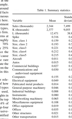
Now, let us turn briefly to the basic characteristics of our regression sample. Table 1 provides summary statistics for the main variables used in the following analysis. One can see here that the firms in this sample are indeed quite large. Sales among these firms averaged roughly $2.3 billion in 1998 and they employed an average of 12,471 workers. These firms collec-tively accounted for about 28% of gross output and 19% of employment in the U.S. private, nonfarm economy. Al-though this sample of firms clearly represents a large fraction
Table 1. Summary statistics
Sales (thousands) 2,344 7,499 —
K (thousands) 2,377 9,055 0.796
L (thousands) 12.471 38.810 0.714
Spike 0.316 0.465 0.025
Size, class 1 0.159 0.222 0.125
Size, class 2 0.193 0.395 0.130
Size, class3 0.221 0.415 0.119
Size, class4 0.212 0.409 0.053
Size, class5 0.215 0.411 0.409
Aircraft 0.011 0.087 0.380
Autos 0.015 0.074 0.258
Commercial buildings 0.027 0.129 0.020
Communications and audiovisual equipment
0.030 0.119 0.028
Computers 0.155 0.222 0.011
Electrical equipment 0.049 0.119 0.015
Fabricated metal products 0.014 0.083 0.023 General-purpose machinery 0.046 0.140 0.009
Industrial buildings 0.088 0.192 0.217
Instruments 0.080 0.141 0.023
Metalworking machinery 0.065 0.187 0.037 Miscellaneous equipment 0.108 0.195 0.021
Office equipment 0.019 0.070 0.011
Offices 0.035 0.146 0.023
Other structures 0.021 0.112 0.006
Other transportation equipment
0.015 0.084 0.011
Software 0.036 0.099 0.044
Special Industrial Machinery 0.156 0.276 0.025
Trucks 0.011 0.074 0.015
Utilities 0.018 0.088 0.002
No. of equipment types 4.563 3.136 —
No. of structure types 1.655 1.167 —
No. of observations 1,650 — —
*Partial correlations controlling for three-digit SIC industry dummy variables.
of economic activity in the United States, it should be noted that the empirical results presented later can only be said to reflect the population of large firms; the relationship between capital composition and productivity for small- to medium-size firms could well be different.
The average firm in our sample invested in five different types of equipment and two different types of structures. On average, sample firms spent 15% of their total capital expen-ditures on computers, 16% on special industry machinery, 11% on miscellaneous equipment, and less than 10% on each other capital type. The lowest average investment share is 1% (for trucks). Interestingly, firms in the sample reported much less investment, on average, on software and communications equipment, each with about 3% of total investment, than on computers. This is likely because firms treat much of their spending on software and communications equipment as inter-mediate expenses rather than capital expenditures. (Note that software that is bundled with, or embedded in, hardware is not counted as a software investment in the ACES.)
It is also worth noting the raw correlations between sales and each of the variables in our regressions. These are shown in the last column of Table 1. Interestingly, computers have virtually no correlation with sales, and software is actually negatively correlated with sales, even though, as shown later, these capital types are positively associated with sales in a multivariate production function regression analysis.
5. RESULTS
5.1 Full Sample Results
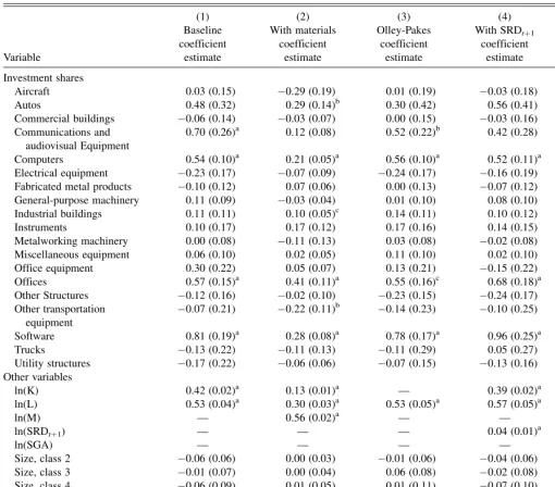
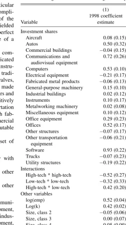
Table 2 presents the main results of the cross-sectional regressions described in Section 3. Each regression is estimated via OLS; standard errors (shown in parentheses in Table 2) are computed using the heteroscedasticity-consistent (Huber-White) variance–covariance matrix. All variables, except where otherwise noted, are 1998 values. I also experimented with using 1999 values instead, while still using 1998 invest-ment shares, as a further attempt to mitigate the possible si-multaneous response of investment shares to contemporaneous productivity shocks in 1999. This would be appropriate if the true capital accumulation process were such that there is a 1 year lag between when investment takes place and when capital is put into use. The 1999 results are quite similar to the 1998 results shown in Table 2 and are provided in Appendix C.
As the production model in Section 3 suggests, it is neces-sary to choose a numeraire capital type whose uj is zero by
definition. I choose special industry machinery and omit its investment share from the regression. The choice of numeraire type is arbitrary and innocuous; it in no way affects the relative marginal products (i.e., the sum or difference of any twouj’s, as
I have verified by omitting alternative capital types). However, the point estimate and statistical significance of eachujapplies
specifically to thejth investment share relative to the particular investment share that is omitted. In the following section, I will back out the actual marginal products of each type, which are not affected by the choice of numeraire.
Before considering the results, a few words regarding the interpretation of these regressions are warranted. The statistical associations that these regressions identify are those between
the investment shares and output conditional on labor and book value of capital (and other control variables). Given that the conventional measure of TFP or MFP is output net of capital quantity (measured either by book value or perpetual inventory accumulation) and labor, each weighted by their production elasticities, these regressions also identify the associations between the investment shares and conventionally measured MFP. However, because this conventional MFP omits the potential additional factor of capital composition/quality, I caution against interpreting the investment share coefficients as associations with true TFP. The validity of interpreting any statistical associations identified in these regressions as causal effects depends on the extent to which unobserved productivity (mit) is controlled for.
Column 1 of Table 2 shows the results from estimating equation (6). I first note that the baseline regression yields an estimate of the elasticity of output with respect to labor of 0.53 (0.04) and the elasticity of output with respect to capital stock of 0.42 (0.02). These elasticity estimates are roughly in line with priors based on U.S. aggregate factor shares, which are about two thirds for labor and one third for capital, although the estimate of labor’s elasticity is somewhat below that implied by factor shares whereas capital’s elasticity estimate is somewhat above. In addition, the elasticity estimates suggest approx-imately constant returns to scale (a^þb^ ¼0:95;which is not significantly different from one). The coefficient on the investment spike variable is positive but insignificant. Firm size, as proxied by employment size, has no significant relationship with productivity in this regression, all else being equal (which is not surprising given that log(Li) is already
included in the regression).
Turning to the key parameters of interest—the estimated coefficients on the type-specific investment shares—the base-line results show that investment in computers, communica-tions equipment, software, and offices is significantly associated statistically, above the 99% level, with output con-ditional on labor and book value of capital. The computer coefficient is 0.54 (SE¼0.10), suggesting that an increase in the computer investment share by 10 percentage points (rela-tive to the omitted capital type) would be expected to be associated with roughly 5% higher output (conditional on total capital stock and labor). The coefficients on communications equipment and software are somewhat higher at 0.70 (0.26) and 0.81 (0.19), respectively. Office building investment has a coefficient of 0.57 (0.15).
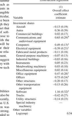
Column 2 shows the results of additionally including (log) materials as a regressor. Note first that, with the exception of just four capital types, the estimated coefficients on the investment shares move closer to zero. This is to be expected. Recall that, in terms of the production function model, the coefficients on the investment shares correspond to auj. The
inclusion of materials reducesa^ by a factor of 3 (from 0.42 to 0.13). Thus, the coefficients on the investment shares should fall by the same proportion. The implied uj’s from this regression
are, in fact, quite similar to those from the first regression, aside from a few statistically insignificant exceptions (aircraft, fab-ricated metal products, instruments, metalworking machinery, and other transportation equipment). The coefficients on the investment shares for computers, software, and offices remain
positive and statistically significant. Investment in autos and industrial buildings becomes positive and significant, and investment in other transportation equipment becomes sig-nificantly negative. Investment in communications equipment goes from being strongly statistically significant to only mar-ginally significant, with apvalue of 0.12. It is worth noting the substantial drop in the coefficients of software and office equipment, the two capital types likely to be the most severely affected by the measurement error associated with misreport-ing of capital expenditures as intermediate expenses. The inclusion of intermediate expenses is likely leading to a mis-attribution of some of the output contribution of these types to intermediate expenses. It is also worth noting that one obtains
very similar results if one replaces 1998 values, for all variables except the investment shares, with 1999 values (see Appendix C). The only notable difference in the 1999 results is that communications equipment becomes strongly statistically significant (positively), and the previous significantly negative effect of other transportation equipment goes away.
The regression underlying column 3 is identical to that of column 1 except that a third-order polynomial (including interactions) in total investment (ln(Ii,98)), book value of capital
(ln(Ki,98)), and firm age are included as a proxy for unobserved
productivity shocks, following Olley and Pakes (1996). Note that in this regression, the coefficient on ln(K) no longer identifies the capital elasticity and hence is not shown. The
Table 2. Production function regressions
Variable
(1) Baseline coefficient
estimate
(2) With materials
coefficient estimate
(3) Olley-Pakes
coefficient estimate
(4) With SRDtþ1
coefficient estimate
(5) With SGA coefficient estimate
Investment shares
Aircraft 0.03 (0.15) 0.29 (0.19) 0.01 (0.19) 0.03 (0.18) 0.16 (0.15)
Autos 0.48 (0.32) 0.29 (0.14)b 0.30 (0.42) 0.56 (0.41) 0.39 (0.27)
Commercial buildings 0.06 (0.14) 0.03 (0.07) 0.00 (0.15) 0.03 (0.16) 0.05 (0.12) Communications and
audiovisual Equipment
0.70 (0.26)a 0.12 (0.08) 0.52 (0.22)b 0.42 (0.28) 0.52 (0.26)b
Computers 0.54 (0.10)a 0.21 (0.05)a 0.56 (0.10)a 0.52 (0.11)a 0.20 (0.09)b
Electrical equipment 0.23 (0.17) 0.07 (0.09) 0.24 (0.17) 0.16 (0.19) 0.20 (0.24) Fabricated metal products 0.10 (0.12) 0.07 (0.06) 0.00 (0.13) 0.07 (0.12) 0.05 (0.11) General-purpose machinery 0.11 (0.09) 0.03 (0.04) 0.01 (0.10) 0.08 (0.10) 0.06 (0.08) Industrial buildings 0.11 (0.11) 0.10 (0.05)c 0.14 (0.11) 0.10 (0.12) 0.01 (0.10)
Instruments 0.10 (0.17) 0.17 (0.12) 0.17 (0.16) 0.14 (0.15) 0.02 (0.18)
Metalworking machinery 0.00 (0.08) 0.11 (0.13) 0.03 (0.08) 0.02 (0.08) 0.03 (0.07) Miscellaneous equipment 0.06 (0.10) 0.02 (0.05) 0.11 (0.10) 0.02 (0.10) 0.04 (0.08)
Office equipment 0.30 (0.22) 0.05 (0.07) 0.13 (0.21) 0.15 (0.22) 0.06 (0.19)
Offices 0.57 (0.15)a 0.41 (0.11)a 0.55 (0.16)c 0.68 (0.18)a 0.09 (0.15)
Other Structures 0.12 (0.16) 0.02 (0.10) 0.23 (0.15) 0.24 (0.17) 0.13 (0.19)
Other transportation equipment
0.07 (0.21) 0.22 (0.11)b 0.14 (0.23) 0.10 (0.25) 0.08 (0.21)
Software 0.81 (0.19)a 0.28 (0.08)a 0.78 (0.17)a 0.96 (0.25)a 0.33 (0.15)b
Trucks 0.13 (0.22) 0.11 (0.13) 0.11 (0.29) 0.05 (0.27) 0.38 (0.24)
Utility structures 0.17 (0.22) 0.06 (0.06) 0.07 (0.15) 0.13 (0.16) 0.67 (0.51) Other variables
ln(K) 0.42 (0.02)a 0.13 (0.01)a — 0.39 (0.02)a 0.27 (0.02)a
ln(L) 0.53 (0.04)a 0.30 (0.03)a 0.53 (0.05)a 0.57 (0.05)a 0.30 (0.04)a
ln(M) — 0.56 (0.02)a — — —
ln(SRDtþ1) — — — 0.04 (0.01)
a
—
ln(SGA) — — — — 0.38
Size, class 2 0.06 (0.06) 0.00 (0.03) 0.01 (0.06) 0.04 (0.06) 0.00 (0.05)
Size, class 3 0.01 (0.07) 0.00 (0.04) 0.06 (0.08) 0.02 (0.08) 0.06 (0.06)
Size, class 4 0.06 (0.09) 0.01 (0.05) 0.01 (0.11) 0.07 (0.10) 0.07 (0.08)
Size, class 5 0.01 (0.13) 0.01 (0.07) 0.07 (0.15) 0.01 (0.15) 0.15 (0.11)
Spike dummy 0.05 (0.04) 0.05 (0.02)a 0.03 (0.04) 0.07 (0.04)c 0.03 (0.03)
Constant 3.35 (0.16)a 2.01 (0.12)a 55.38 (133.6) 3.18 (0.18)a 2.53 (0.14)a
No. of observations 1,651 1,409 1,457 1,201 1,394
R2 0.8959 0.9780 0.9201 0.9204 0.9247
NOTE: These regressions also include three-digit SIC industry dummies and state dummies, although as a result of confidentiality concerns, the coefficients on these dummies are not shown. In addition, column 3 contains all terms, including interactions, of a third-order polynomial in (I, K, and age).
Robust standard errors are shown in parentheses. aSignificant at the 99% level.
bSignificant at the 95% level.
cSignificant at the 90% level.
addition of this polynomial has very little effect on the results relative to column 1. The coefficients on the investment shares for computers, software, and offices are approximately the same and remain highly statistically significant. The coef-ficient on communications equipment falls noticeably (from 0.70 to 0.52), although the decline is not statistically significant and the coefficient remains statistically significantly different from zero. In addition, as with the other specifications, esti-mating this regression using 1999 values for all variables except the 1998 investment shares yields very similar results (see Appendix C)—in particular, the coefficients for com-puters, software, communications equipment, and offices are roughly the same magnitude and are statistically significant. This is notable because, as mentioned in Section 3, one potential concern with applying the Olley-Pakes technique in this context is that it assumes firms do not change their investment mix in response to the transmitted productivity shock. If this were not the case, the contemporaneous invest-ment shares, unlike the predetermined, lagged investinvest-ment shares, would partially reflect the productivity shock, and thus the coefficients on the investment shares would be significantly different when they are lagged versus contemporaneous.
Column 4 presents the results of adding the 1-year lead of the Solow residual (srdi,99) to the baseline regression. Compared
with the baseline regression results, this addition has a small but notable effect on the estimated investment share coef-ficients. Investment in computers, software, and offices remain positively and significantly associated with labor productivity. The coefficient on communication equipment falls from 0.70 to 0.42 and is no longer statistically significant at the 10% level (the p value is 0.12). I note, though, that when I repeat this regression using 1999 data (except the 1998 investment shares), communications equipment is again statistically sig-nificant at the 10% level (with a coefficient of 0.37 [0.20]; see Appendix C).
In the regression underlying column 5, I add to the baseline regression the log of SGA as a proxy for organizational capital, following Lev and Radhakrishnan (2005). As discussed in Section 3, including SGA as an additional regressor in our main production function regression serves to control partially for the unobserved, transmitted productivity components. Note first that the estimated elasticity of output with respect to organizational capital (SGA) is 0.38. As is to be expected under a prior of approximately constant returns to scale (with labor, physical capital, and organizational capital as production factors), the labor and (physical) capital elasticities fall accordingly to 0.30 and 0.27, respectively. The implied returns to scale parameter, at 0.95, is unchanged from the baseline results (column 1).
Given the decline inaof roughly a third, the coefficients on the investment shares should also be expected to decline by about a third relative to the baseline results, and, in general, this appears to be case. Thus, for the most part, the implied relative productivities are unaffected by the inclusion of SGA. The key exception is that the coefficient on office buildings falls to near zero and is statistically insignificant. Thus, it appears that the previous statistical association between office building investment and output was spurious and driven by the fact that office building investment is highly correlated with organiza-tional capital that has an independent positive effect on
con-ventionally measured MFP. It is worth noting that the coefficients on computers and software also fall by more than expected (they each decrease by roughly 60%), although they remain positive and statistically significant. This implies some of the previous association between computers and software and productivity likely was the result of the fact that these types of capital are important complements with organizational capital. (Interestingly, the coefficient on office equipment, another cat-egory one would expect to be highly correlated with organiza-tional capital, also declines considerably, from 0.30 to –0.06.)
5.2 Interpretation of Results
In Section 3, I showed that the coefficient on a particular investment share, auj, can be interpreted as the (ex-post)
marginal product of the capital type (relative to the omitted type), adjusted for its relative depreciation rate, multiplied by the elasticity of capital in the production function:
auj¼a Fj=F01 d=dj
, wheredanddjare the
depreci-ation rates for total capital and type-j capital, respectively. Under the neoclassical assumption that firms equilibrate mar-ginal products to factor prices (Fj/F0¼cj/c0), this coefficient
should thus equala cj=c01 d=dj, wherecjandc0are the
implicit rental prices (also known as user costs) for type-jand type-0 capital, respectively. The BLS provides estimates of depreciation rates, as well as estimates of rental prices, at a detailed capital-type level (which has a many-to-one mapping to our 20-type level). The data are widely used by researchers and other government agencies in the construction of capital stock data. In general, the rental prices are estimated from data on rental rates for specific capital goods observed in capital rental markets. The depreciation rates are estimated from pri-ces of used capital assets observed in secondary markets. Using our estimate of a, along with the BLS measures ofd anddj,
one can thus back out the implied ratio of marginal products between capital type j and the numeraire capital type. Fur-thermore, taking the BLS estimate of the user cost of the numeraire type—in our case, special industry machinery—as approximately equal to the marginal product of this capital type, one can back out the marginal product (per dollar of capital stock) for every capital type.
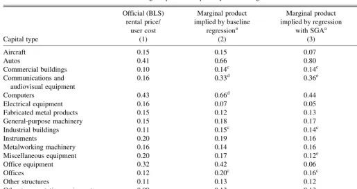
Table 3 shows the marginal products for each type of capital implied by our regression results. Column 1 shows the rental prices for 1998 provided by the BLS. Column 2 gives the marginal products implied by the baseline regression results (column 1 of Table 2), whereas column 3 gives the marginal products implied by the regression that controls for organiza-tional capital as proxied by SGA (column 5 of Table 2). The letters next to each implied marginal product indicate the degree to which it is significantly different statistically from the BLS estimated rental price. The confidence inter-vals here assume that everything in the expression
a Fj=F01 d=dj is known with certainty except the estimated parameter,Fj.
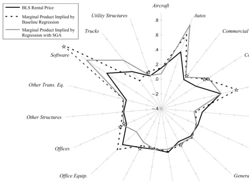
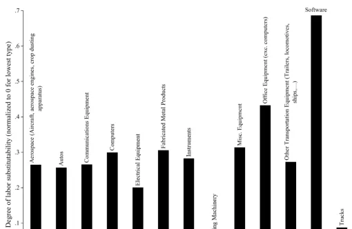
To aid in the comparison, the implied marginal products and BLS rental prices also are shown graphically with the radial chart in Figure 1. Each spoke in this chart corresponds to a specific capital type. The points on the spokes that are con-nected by the solid black lines correspond to the BLS rental
prices given in column 1 of Table 3. The points connected by the dashed black lines correspond to the baseline implied marginal products (column 2), whereas the points connected by the solid gray lines correspond to the implied marginal prod-ucts shown in column 3. Stars indicate marginal product esti-mates that are statistically significantly different from the corresponding BLS rental price.
For most capital types, the marginal product implied by the baseline regression is strikingly similar to the BLS rental price. For instance, for miscellaneous equipment, metalworking machinery, instruments, general-purpose machinery, fabricated metal products, other structures, and aircraft, the difference between the implied marginal product (from the baseline pro-duction function estimation) and the BLS rental price is within just three percentage points. For several capital types, however, the implied marginal product is found to be significantly (statistically and economically) higher than the BLS estimate of the rental price. In particular, using the baseline production function estimates, computers are found to have had an ex-post marginal product of 66% in 1998, compared with the BLS’ estimated rental price of 43%. Communications equipment had an estimated marginal product of 33%, compared with a 16% estimated rental price. Software also had an estimated marginal product above the BLS’ rental price: 119% versus 48%.
The baseline implied marginal products for commercial buildings, industrial buildings, offices, utility structures, and other structures are also statistically significantly higher than
their BLS rental prices. However, this result should be viewed with caution. First, although statistically significant, the dif-ferences for these types are small (ranging from four to eight percentage points). Second, as noted earlier, structures invest-ment tends to be infrequent and heavily concentrated among industries. Therefore, the estimated coefficients on their investment shares may, to some extent, reflect industry effects not picked up by the three-digit industry dummies included in the regressions.
The marginal products implied by the regression that includes SGA also is generally quite similar to the BLS rental prices. Looking at Figure 1, the primary differences that stand out are for communications equipment, software, and autos (with implied marginal products that are substantially above their rental prices) and office equipment (with an implied marginal product sub-stantially below its rental price). However, only the difference for communications equipment is statistically significant.
As discussed in Section 3, there are a number of possible reasons why the estimated ex-post marginal product for a capital good could be different than its rental price. First, there could be adjustment costs, including learning costs, that dis-proportionately affect particular capital goods (David 1990; Cummins and Dey 1998). Second, certain capital goods may be associated with unobserved organizational coinvestments. For example, a number of authors have argued that organ-ization coinvestments, such as human resource management programs, training programs, quality control systems, and so
Table 3. Marginal products implied by baseline regression results
Capital type
Official (BLS) rental price/
user cost (1)
Marginal product implied by baseline
regressiona (2)
Marginal product implied by regression
with SGAa (3)
BLS depreciation
rateb (4)
Aircraft 0.15 0.15 0.07 0.08
Autos 0.41 0.66 0.80 0.30
Commercial buildings 0.10 0.14c 0.14c 0.01
Communications and audiovisual equipment
0.16 0.33d 0.36e 0.08
Computers 0.43 0.66d 0.44 0.27
Electrical equipment 0.16 0.07 0.05 0.09
Fabricated metal products 0.15 0.12 0.13 0.07
General-purpose machinery 0.15 0.18 0.17 0.08
Industrial buildings 0.11 0.15c 0.14c 0.02
Instruments 0.20 0.19 0.16 0.12
Metalworking machinery 0.16 0.14 0.16 0.09
Miscellaneous equipment 0.20 0.17 0.12e 0.13
Office equipment 0.32 0.42 0.06 0.26
Offices 0.12 0.20c 0.16c 0.03
Other structures 0.11 0.13 0.12 0.04
Other transportation equipment 0.09 0.13 0.13 0.04
Software 0.48 1.19c 0.81 0.37
Trucks 0.24 0.08 0.43 0.14
Utility structures 0.07 0.13c 0.08 0.02
aCalculated as: [(inv. share coefficient/capital elasticity)
3(BLS relative depreciation rate)þ1]3(BLS rental price for special industry machinery). The BLS estimate of the user cost for special industry machinery is 0.1449283.
bThe BLS estimate of the depreciation rate for total capital is 0.0980.
c–eImplied marginal product is significantly different than official (BLS) rental price (assuming only source of randomness in formula in footnote a comes from the inv. share coefficient).
cSignificant at the 99% level.
dSignificant at the 95% level.
eSignificant at the 90% level.
on, contribute to productivity and are facilitated by ICT capital. Third, as a result of uncertainty regarding the rate of return on capital investments, there could be systematic expectational errors by firms that may be more severe for certain capital goods. For instance, it is often posited that firms systematically overinvested in communications equipment in the late 1990s. Interestingly, though, I find that, in fact, the marginal product on communications equipment during this period was actually above its implicit rental price.
6. COMPLEMENTARITIES AND
SUBSTITUTABILITIES
6.1 Among Capital Types
The results presented thus far establish that the standard measure of capital stock used in micro level production func-tion estimafunc-tion does not adequately account for capital mix. However, these results do not shed light on the fundamental question of whether it is at all possible to express capital services as a single aggregate. As discussed in Section 3, the ability to express a firm’s total capital services with a single measure, even if that measure weights heterogeneous capital goods by their relative marginal products, requires that (1)
individual capital services each be weakly separable with labor (Solow 1955–1956) and (2) that their services be expressed in common units (Fisher 1965). These two conditions together require that different capital services be perfectly substitutable. These conditions have long been viewed by many economists as unrealistic. Solow himself, referring to the first of the two, commented that it ‘‘will not often be even approximately sat-isfied in the real world,’’ (Solow 1955–1956, p. 103).
The hypothesis of perfect substitutability can be straight-forwardly tested with the ACES data. Specifically, one can test whether certain ‘‘bundles’’ (e.g., pairs, triples, quadruples) of different types of capital have an impact on output above and beyond the individual effects that each type of capital has. In the case of pairs, this is a test of whether the cross-partial derivative for any pair of capital goods is equal to zero:Fjk¼0
forj6¼k.
Starting with the baseline production function regression discussed earlier, I add interactions of investment shares between every possible pair (dyad) of capital types in our data. With 20 types, this amounts to 190 interactions. The results (available upon request) are not shown for space consid-erations. I note first that the investment shares for computers, communications equipment, software, and office buildings remain statistically significant, even after the inclusion of these
Figure 1. Implied marginal products and BLS rental prices.