Full Terms & Conditions of access and use can be found at
http://www.tandfonline.com/action/journalInformation?journalCode=ubes20
Download by: [Universitas Maritim Raja Ali Haji] Date: 11 January 2016, At: 22:38
Journal of Business & Economic Statistics
ISSN: 0735-0015 (Print) 1537-2707 (Online) Journal homepage: http://www.tandfonline.com/loi/ubes20
Testing Predictive Ability and Power
Robustification
Kyungchul Song
To cite this article: Kyungchul Song (2012) Testing Predictive Ability and Power Robustification, Journal of Business & Economic Statistics, 30:2, 288-296, DOI: 10.1080/07350015.2012.663245
To link to this article: http://dx.doi.org/10.1080/07350015.2012.663245
View supplementary material
Accepted author version posted online: 10 Feb 2012.
Submit your article to this journal
Article views: 177
Testing Predictive Ability and Power
Robustification
Kyungchul S
ONGDepartment of Economics, University of British Columbia, Vancouver BC V6T 1Z1, Canada ([email protected])
One of the approaches to compare forecasting methods is to test whether the risk from a benchmark prediction is smaller than the others. The test can be embedded into a general problem of testing inequality constraints using a one-sided sup functional. Hansen showed that such tests suffer from asymptotic bias. This article generalizes this observation, and proposes a hybrid method to robustify the power properties by coupling a one-sided sup test with a complementary test. The method can also be applied to testing stochastic dominance or moment inequalities. Simulation studies demonstrate that the new test performs well relative to the existing methods. For illustration, the new test was applied to analyze the forecastability of stock returns using technical indicators employed by White.
KEY WORDS: Data snooping; Inequality restrictions; One-sided sup tests; Power robustification; Reality check.
1. INTRODUCTION
Comparing multiple forecasting methods is important in prac-tice. Diebold and Mariano (1995) proposed tests comparing two forecasting methods, and West (1996) offered a formal analysis of inference based on out-of-sample predictions. White (2000) developed a general testing framework for multiple forecast-ing models, and Hansen (2005) developed a way to improve the power of the tests in White (2000). Giacomini and White (2006) introduced out-of-sample predictive ability tests that can be applied to conditional evaluation objectives. There also has been interest in evaluation of density forecasts in the literature. For earlier contributions see Diebold, Gunther, and Tay (1998); Christoffersen (1998); and Diebold, Hahn, and Tay (1999); and for more recent researches, see Amisano and Giacomini (2007) and Bao, Lee, and Salto˘glu (2007), among others. For a general survey of forecast evaluations, see West (2006) and references therein.
This article’s main focus is on one-sided sup tests of predic-tive ability developed by White (2000) and applied by Sulli-van, Timmermann, and White (1999). A one-sided sup test is based on the maximal difference between the benchmark and the candidate forecast performances. Hansen (2005) demon-strated that the one-sided sup tests are asymptotically biased, and suggested a way to improve their power. His approach is general and, in fact, related to some later literature on testing moment inequalities such as Andrews and Soares (2007); Bugni (2010); Andrews and Shi (2011); and Linton, Song, and Whang (2010).
This article generalizes the observation by Hansen (2005), and proposes a method to robustify the local asymptotic power behavior. The main idea is to couple the one-sided sup test with a complementary test that shows better power proper-ties against alternative hypotheses under which the one-sided sup test performs poorly. For a complementary test, this article adopts a symmetrized test statistic used by Linton, Maasoumi, and Whang (2005) for their stochastic dominance tests. This article calls this coupled test a hybrid test, as its power prop-erties are intermediate between those of the one-sided sup test
and the symmetrized test. As this article demonstrates, one can easily apply a bootstrap procedure to obtain approximate crit-ical values for the hybrid test by using the existing bootstrap procedures.
Many recent researchers have focused on the testing problem of inequality restrictions that hold simultaneously under the null hypothesis. See, for example, Hansen (2005), Andrews and Soares (2007), Bugni (2010), Canay (2010), Linton et al. (2009), Andrews and Shi (2010), and references therein. This article’s approach contrasts with the proposals mentioned above. In the context of testing predictive ability, these proposals improve the finite sample power properties of the test by eliminating fore-casting methods that perform poorly beyond a threshold when computing a critical value. Since using a fixed threshold makes the test asymptotically invalid, the threshold is chosen to be less stringent as the sample size becomes larger, satisfying certain rate conditions. On the other hand, this article’s approach mod-ifies the sup test to have a better local power against alternatives that the original test is known to have weak power, and hence using a sequence of thresholds is not required.
A test of such inequality restrictions is said to be asymp-totically similar on the boundary, if the asymptotic rejection probability remains the same whenever any of the inequality re-strictions is binding under the null hypothesis. A recent article by Andrews (2011) showed an interesting result that a test of such inequality restrictions that is asymptotically similar on the boundary has poor power properties under general conditions. Like the work mentioned previously, the hybrid test of this ar-ticle improves power properties by alleviating asymptotic bias of the one-sided test against certain alternatives, but does not eliminate entirely the asymptotic nonsimilarity of the one-sided test. Hence the test is not subjected to the poor power problem pointed out by Andrews (2011).
© 2012American Statistical Association Journal of Business & Economic Statistics April 2012, Vol. 30, No. 2 DOI:10.1080/07350015.2012.663245
288
Song: Testing Predictive Ability and Power Robustification 289
Here, the performance of the hybrid test is investigated through Monte Carlo simulation studies. Overall, the new test performs as well as the tests of White (2000) and Hansen (2005), and in some cases, performs conspicuously better.
This article applies the hybrid test to investigate the fore-castability of S&P500 stock returns by technical indicators in a spirit similar to the empirical application in White (2000). Considering the periods from March 28, 2003, through July 1, 2008, the empirical application tests the null hypothesis that no method among the 3654 candidate forecasting methods consid-ered by White (2000) outperforms the benchmark method based on sample means. The hybrid test has conspicuously lowerp -values than the tests of Hansen (2005) and White (2000). A brief explanation behind this finding is provided in the article.
The article is organized as follows. The next section discusses poor power properties of one-sided sup tests. Section 3 intro-duces a general method of coupling the one-sided test with a complementary one. Sections 4 and 5 present and discuss results from Monte Carlo simulation studies, and an empirical applica-tion on stock returns forecastability. Secapplica-tion 6 concludes.
2. TESTING PREDICTIVE ABILITY AND ASYMPTOTIC BIAS
In producing a forecast, one typically adopts a forecasting model, estimates the unknown parameter, and then produces a forecast using the estimated forecasting model. Since a fore-casting model and an estimation method constitute eventually a single map that assigns past observations to a forecast, we follow Giacomini and White (2006) and refer to this map gener-ically as aforecasting method. Given informationFT at time T, multiple forecasting methods are generically described by mapsϕm, m∈M, fromFT to a forecast, whereM⊂Rdenotes
the set of the indices for the forecasting methods. The setM can be a finite set or an infinite set that is either countable or uncountable. Let(m) denote the risk of prediction based on themth candidate forecasting method, and(0) the risk of pre-diction based on a benchmark method. Then the difference in performance between the two methods is measured by
d(m)≡(0)−(m).
We are interested in testing whether there is a candidate fore-casting method that strictly dominates the benchmark method. The null and the alternative hypotheses are written as:
H0:d(m)≤0, for allm∈M,and (1) H1:d(m)>0, for somem∈M.
Let us consider some examples of(m).
Example 1 [Point Forecast Evaluated With the Mean Squared Prediction Error (MSPE)]. Suppose that there is a time se-ries {(Yt,X⊤t )}∞t=1, where we observe part of it, say, FT ≡ mth forecasting model known up toβ. Since ˆβm,T is estimated
usingFT, we can write ˆβm,T =τm(FT) for some mapτm. When
The expectation above is with respect to the joint distribution of variables constituting informationFTandYT+τ.
Example 2 (Density Forecast Evaluated With the Expected Kullback–Leibler Divergence). Let {(Yt,X⊤t )}∞t=1 and FT ≡
ing themth forecasting method and informationFT. Following
Bao et al. (2007), we may take the expected Kullback–Leibler divergence as a measure of discrepancy between the forecast densityfm,T+τ(·;FT) and the actual densityfT+τ(·):
does not depend on the choice of a forecasting method, we focus on the second part only in comparing the methods. Hence we take
Example 3 (Conditional Forecast Evaluated With the MSPE). Giacomini and White (2006) proposed a general frame-work of testing conditional predictive abilities. Let{(Yt,X⊤t )}∞t=1
and define the conditional MSPE
(m|GT)=E[{YT+τ−ϕm(FT)}2|GT],
whereGT is part of the informationFT. For example, the
fore-cast is generated from ˆYT(m)+τ =fm(FT; ˆβm) as in Example 1.
Then the null hypothesis of interest is stated as d(m|GT)≤0
for all m∈M, where d(m|GT)=(0|GT)−(m|GT), with (0|GT) denoting the benchmark method’s conditional MSPE.
The null hypothesis states that regardless of how the informa-tion GT realizes, the performance of the benchmark method
dominates all the candidate methods. As in Giacomini and White (2006), we choose an appropriate test function h(GT), and focus on testing (1) with d(m)=(0)−(m), where
(m)≡E[h(GT){YT+τ−ϕm(FT)}2].A remarkable feature of
Giacomini and White’s (2006) study is that their testing proce-dure is designed to capture the effect of estimation uncertainty when a fixed sample size is used for the estimation even as
T → ∞. This feature is also accommodated in this article’s framework.
The usual method of testing (1) involves replacing (m) by an estimator ˆ(m) and constructing an appropriate test us-ing ˆd(m)=ˆ(0)−ˆ(m). For Examples 1–3 above, we can
construct the following:
ˆ
(m)= T 1 −R+1
T
t=R
{Yt+τ−fm(Ft; ˆβm,t)}2(Example 1),
ˆ
(m)= − 1
T −R+1
T
t=R
log(fm,t+τ(Yt+τ;Ft))
(Example 2), and
ˆ
(m)= T 1 −R+1
T
t=R
h(Gt){Yt+τ−fm(Ft; ˆβm,t)}2
(Example 3),
where the periodsR+τ, . . . , T +τ are target periods of fore-cast. [For obtainingfm,t+τ(Yt+τ;Ft) in Example 2, see Bao et al.
(2007) and Amisano and Giacomini (2007) for details.] Letn denote the number of the time series observations used to pro-duce ˆd(m). The random quantity ˆd(m) is viewed as a stochastic process indexed bym∈M, or briefly a random function ˆd(·) on M. The main assumption for this article is the following:
Assumption 1. There exists a Gaussian processZwith a con-tinuous sample path onMsuch that
√
n{dˆ(·)−d(·)} =⇒ Z(·), asn→ ∞, (2)
where =⇒denotes weak convergence of stochastic processes onM.
When M= {1,2, . . . , M}, Assumption 1 is satisfied if for ˆ
d=[ ˆd(1), . . . ,dˆ(M)]⊤andd=[d(1), . . . , d(M)]⊤,
√
n(dˆ−d)→d Z≡[Z(1), . . . , Z(M)]⊤ ∼N(0, ) (3)
for a positive semidefinite matrix(i.e., for allt∈RM t⊤Zis zero ift⊤t=0, andt⊤Z∼N(0,t⊤t) ift⊤t>0). There-fore, the predictive models are allowed to be nested as in White (2000) and Giacomini and White (2006). In the situation where the forecast sample is small relative to the estimation sample, the estimation error in ˆβm,t becomes irrelevant. On the other
hand, in the situation where parameter estimation uses a rolling window of observations with a fixed window length as in Gia-comini and White (2006), the estimation error in ˆβm,tremains
relevant in asymptotics. Assumption 1 accommodates both the situations.
Assumption 1 also admits infinite M. The case arises, for example, when one tests the conditional MSPE as in Example 3 usinga class oftest functions instead of using a single choice ofh[e.g., Stinchcombe and White (1998)]. In this case,Malso includes the indices of such a class of test functions.
However, Assumption 1 excludes the case where (·) is a regression function of a continuous random variable and ˆ(·) is its nonparametric estimator. While such a case arises rarely in the context of testing predictive abilities, it does in the context of testing certain conditional moment inequalities [e.g., Lee, Song, and Whang (2011)].
We first show that tests based on the one-sided sup test statis-tic,
TK ≡√nsup
m∈M ˆ
d(m), (4)
are asymptotically biased. To define a local power function, we introduce Pitman local alternatives in the directiona:
d(m)=a(m)/√n. (5)
The directionarepresents how far and in which direction the alternative hypothesis is from the null hypothesis. For example, suppose thatM= {1,2, . . . ,}, that is, we have M candidate forecasting methods, and consider an alternative hypothesis with asuch thata(1)=c >0 anda(m)=0 for allm=2, . . . , M. The alternative hypothesis in this case is such that the first forecasting method (m=1) has a risk smaller than that of the benchmark method byc/√n.
Proposition 1. Suppose that Assumption 1 holds. Then for anycα >0 with limn→∞P{TK > cα} ≤αunderH0, there
ex-ists a mapa:M→Rsuch that under the local alternatives of type (5),
lim
n→∞Pa
TK > cα
≤α−+ε,
wherePa denotes the sequence of probabilities under (5) and =P{supm∈MZ(m)> cα} −infm∈MP{Z(m)> cα}.
Proposition 1 shows that the sup test of (1) has a severe bias whenis large. Proposition 1 relies only on generic features of the testing setup such as (1) and (2), and hence also applies to many inequality tests in contexts beyond those of testing predictive abilities. A general version of Proposition 1 and its proof is found in the supplemental note.
The intuition behind Proposition 1 is simple. Suppose that
P{supm∈MZ(m)> cα} =α. Then, the asymptotic power
un-der the local alternatives withais given byP{supm∈MZ(m)+ a(m)> cα}. Suppose we take a(m) of the form in Figure 1
witha(m0) positive but close to zero, whereas for otherm’s, a(m) is very negative. Then supm∈MZ(m)+a(m) is close toZ(m0)+a(m0) with high probability. Sincea(m0) is close to
zero,
P
sup
m∈M
Z(m)+a(m)> cα
≤P{Z(m0)> cα} +ε
Figure 1. Illustration of an alternative hypothesis associated with low power. Recall that whena(m) takes a positive value for somem, the situation corresponds to an alternative hypothesis. Whena(m) is highly negative atm’s away fromm0 anda(m0) is positive but close
to zero, supm∈MZ(m)+a(m) is close toZ(m0) with high probability,
making it likely that the rejection probability is belowα.
Song: Testing Predictive Ability and Power Robustification 291
for small ε >0. Since typically P{Z(m0)> cα}< P{supm∈MZ(m)> cα} =α, we obtain the asymptotic bias
result.
3. POWER ROBUSTIFICATION VIA COUPLING
3.1 A Complementary Test
The previous section showed that the sup test has very poor power against certain local alternatives. This section proposes a hybrid test that improves power against such local alternatives. Given ˆd as before, we construct another test statistic:
TS=minmax
m∈M ˆ
d(m),max
m∈M(− ˆ
d(m)). (6)
This type of test statistic was introduced by Linton et al. (2005) for testing stochastic dominance. For testing (1),TSis comple-mentarytoTK in the sense that usingTS results in a greater
power against such local alternatives that the testTKperforms
very poorly.
To illustrate this point, let M= {1,2} and X1 and X2 be given observations which are positively correlated and jointly normal with a mean vectord=[d(1), d(2)]⊤.We are interested in testing
H0 :d(1)≤0 and d(2)≤0, against H1 :d(1)>0 or d(2)>0.
Consider TK
=max{X1, X2} and TS=min{max{X1, X2},
max{−X1,−X2}}. Complementarity between TK and TS is
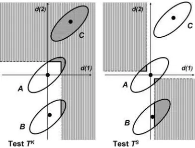
illustrated in Figure 2 in a form borrowed from Hansen (2005). The ellipses in Figure 2 indicate representative contours of the joint density ofX1andX2,each corresponding to different
dis-tributions denoted byA,B, andC. WhileArepresents the null hypothesis under a least favorable configuration (LFC), that is,
Figure 2. Complementarity ofTKandTS: Both panels depict three
ellipses that represent contours from the joint density of (X1, X2) under
different probabilities. Contour A corresponds to the least favorable configuration under the null hypothesis, and contours B and C different probabilities under the alternative hypothesis. The lighter gray areas on both panels represent the rejection regions of the tests. Under the alternative hypothesis of type C, the testTK has a better power than
the testTS, while under the alternative hypothesis of type B, the test TShas a better power than the testTK(as shown by a larger dark area
within the contour B for the testTSthan for the testTK).
d(1)=d(2)=0,BandCrepresent alternative hypotheses. Un-derB,the rejection probability of the testTKis lower than that
underA,implying the biasedness of the test. (This is illustrated by the dark area in ellipsisBin the left panel which is smaller than the dark area in ellipsisAin the same panel.) However, the rejection probability of the testTS againstBis better than the
testTK as indicated by a larger dark area in the ellipsisBon
the right panel than that on the left panel. (This contrast may be less stark whenX1andX2are negatively correlated.) Hence
againstB,testTS has a better power than testTK.This order of performance is reversed in the case of an alternativeCwhere the testTS has a power close to zero, while the testTK has a power close to 1.
3.2 Coupling
We construct a hybrid test by coupling TK and TS. For a
given levelα∈[0,1] andγ ∈[0,1],we define a hybrid test of (1) as follows:
RejectH0 ifTS> cSα(γ) or (7)
ifTS≤cαS(γ) andTK > cαK(γ),
wherecSα(γ) andcKα(γ) are threshold values such that
limn→∞P{TS> cSα(γ)} =αγ
and
limn→∞P{TS≤cSα(γ), T K > cK
α(γ)} =α(1−γ).
The hybrid test runs along a locus betweenTK andTSas we
moveγbetween 0 and 1.Whenγis close to 1, the hybrid test be-comes close toTS, and whenγis close to zero, it becomes close
toTK.The power-reducing effect of the negativity ofd(m) for
mostm’s on the testTKis counteracted by the power-enhancing
effect of the positivity of−d(m) for mostm’s on the testTS.
By coupling withTS,the hybrid test shares this counteracting
effect. Without reasons to do otherwise, this article proposes usingγ =1/2.
Critical values can be computed using bootstrap. First, we simulate the bootstrap distributionP∗of (TS, TK) by generating (TbS∗, TbK∗)Bb=1,whereBdenotes the bootstrap number. [When
observations are stationary series, this can be done using the stationary bootstrap method of Politis and Romano (1994). See also for details White (2000) and Hansen (2005).] Using the empirical distribution of{TS∗
b } B
b=1, we first computec S∗
α (γ) such
that
1
B B
b=1
1{TbS∗ > cαS∗(γ)} =αγ. (8)
Given cS∗
α (γ), we can take cαK∗(γ) to be the (1−α(1−γ
))-percentile of the bootstrap series,TK∗
b ·1{TbS∗ ≤cSα∗(γ)}, b=
1, . . . , B.
The method of coupling hardly entails additional computa-tional cost. The computacomputa-tional cost in most cases arises when one computes ˆd∗(m) using the bootstrap samples, which is a step common in other bootstrap-based tests. Once ˆd∗(m) is com-puted, finding TbK∗ and TbS∗ and obtaining bootstrap critical values are straightforward.
We define thep-values for the test as follows:
the hybrid test does not reject the null hypothesis. In practice, one starts from α=0 and increases along a grid point until
TS> cS∗
α (γ) or TK > cαK∗(γ). Since bootstrap statistics T K∗
b
andTbS∗ have already been computed, the grid search can be done very fast.
3.3 A Recursive Search for a Better Forecasting Method
When the search for a better forecasting method is an ongoing process with candidate models continuing to expand at each search, it is convenient to have a search algorithm that properly takes account of the past searches. White (2000) proposed such an algorithm for practitioners. In this section, we similarly offer the method of recursive search based on the hybrid test.
Given bootstrap versions {dˆ∗
b(m)}Bb=1, m=1, . . . , M, and
a consistent asymptotic variance estimator ˆω2(m) such that
√
n( ˆd(m)−d(m)}/ωˆ(m)→d N(0,1), we define
˜
db∗(m)=dˆb∗(m)−dˆ(m). (10)
[One may construct ˆω2(m) using an HAC
(heteroscedasticity-autocorrelation consistent) type estimator as done in Hansen (2005), p. 372.] Now, the recursive search that this article sug-gests proceeds as follows:
Step 1. For model 1, compute dˆ(1)=ˆ(0)−ˆ(1), its asymptotic variance estimator ωˆ2(1), and the
boot-strap version {dˆ∗ asymptotic variance estimator ˆω2(m), and the bootstrap version
{dˆb∗(m)}Bb=1. SetT
At each Step m, the bootstrap p-value can be computed as in (9), where we replaceTS∗
The recursive search at Stepmcarries along the history of previous searches done using the same data. Similarly as in the spirit of White (2000), we emphasize that as for the previous searches, the recursive search at any Stepmrequires only knowl-edge ofTmK−1,+, TmK−1,−, {TmK−∗1,+,b}Bb=1,and{TmK−∗1,−,b}Bb=1. In other words, one does not need to know the entire history of the searches and performances, before one turns to the next search.
4. MONTE CARLO SIMULATIONS
4.1 Data-Generating Processes and Three Tests
The first part of the simulations focuses on the simulation design considered by Hansen (2005) and compares three types of tests, a test of White (2000) (Reality Check: RC), a test of Hansen (2005) (Superior Predictive Ability: SPA), and this article’s proposal (Hybrid Test: Hyb). The second part considers local alternatives that are different from those of Hansen (2005). Suppose that ˆYT(m)+τ is aτ-step ahead forecast ofYT+τ using
the mth method. The relative performance is represented by
L(YT+τ,Yˆ
a benchmark method. The risk difference is given byd(m)=
E[L0,T −Lm,T]. alternatives with local positivity and alternatives with both lo-cal positivity and lolo-cal negativity. These two schemes are to be specified in Sections 4.2.1 and 4.2.2 later.
First, consider two test statistics, one according to White (2000) and the other according to Hansen (2005):
TRC=√nmax
To construct critical values, we generated the bootstrap ver-sion{dˆ∗
b(m)}Bb=1, b=1,2, . . . , B,of ˆd(m) by resampling from
observations{L0,t−Lm,t}tn=1 with replacement, and let ˜db∗(m)
be as defined in (10). We constructed
Reality Check Test (RC) :
RejectH0 ifTRC> cRCα ∗and
Superior Predictive Ability Test (SPA) :
RejectH0 ifTSPA> cαSPA∗, ing on whether ˆd(m) is close to the boundary of the inequalities or not. The selective recentering is done to improve the power of the test by weeding out the forecasting methods that perform badly.
For the hybrid test which is the main proposal of this article, define first the complementary test statistic:
TS=√nmin
Song: Testing Predictive Ability and Power Robustification 293
As forTK, we takeTK
=TSPAdefined in (11). As for critical
values, construct
In the simulation studies, the sample sizenwas 200 and the number of Monte Carlo simulations and the bootstrap Monte Carlo simulations 2000. The number (M) of candidate forecast-ing methods was chosen from{50,100}.
4.2 Alternative Hypotheses
4.2.1 Alternatives With Local Positivity. Following Hansen (2005), we first consider the following alternatives with
λ(m): method (m=0). Their relative performance is ordered asM≺ M−1≺ · · · ≺2.
When λ(1)=0, no alternative forecasting method strictly dominates the benchmark method, representing the null hypoth-esis. Whenλ(1)< λ(0)=0,the method 1 performs better than the benchmark method, representing the alternative hypothesis. The magnitudeρ controls the extent to which the inequalities
λ(m)≥λ(0)=0, m=2, . . . , M,lie away from binding. When
ρ=0,the remaining inequalities for methods 2 throughMare binding, that is,d(m)=0 for allm=2, . . . , M.
Tables1 and2 show the empirical size of the tests under DGP A. The results show that the test RC has lower Type I error as the design parameterρ increases. For example, when
ρ=2,the rejection probability of the test RC is 0.0005 when the nominal size is 5% andM=50.This extremely conserva-tive size of the test RC is significantly improved by the test SPA of Hansen (2005) which shows the Type I error of 0.0180. This improvement is made through two channels: the normalization by ˆω(m) of the test statistic and the trimming of poorly
per-Table 1. Empirical size of tests of predictive abilities under DGP A (M=50, n=200)
α=0.05 α=0.10
ρ λ(1) RC SPA Hyb RC SPA Hyb
0 0 0.0520 0.0615 0.0620 0.1005 0.1180 0.1160 2 0 0.0005 0.0180 0.0365 0.0045 0.0330 0.0530 3 0 0.0005 0.0125 0.0230 0.0005 0.0210 0.0425 4 0 0.0000 0.0105 0.0220 0.0000 0.0230 0.0350
Table 2. Empirical size of tests of predictive abilities under DGP A (M=100, n=200)
α=0.05 α=0.10
ρ λ(1) RC SPA Hyb RC SPA Hyb
0 0 0.0505 0.0710 0.0610 0.1060 0.1290 0.1210 2 0 0.0010 0.0125 0.0280 0.0040 0.0245 0.0485 3 0 0.0005 0.0080 0.0205 0.0015 0.0200 0.0355 4 0 0.0000 0.0120 0.0220 0.0015 0.0230 0.0315
forming forecast methods. The hybrid approach shows a further improvement over the test SPA, yielding Type I error of 0.0365 in this case.
Tables 3 and 4 show the power of the three tests. As for Hyb, the rejection probability is slightly lower than that of SPA in the case ofρ=0.It is interesting to see that the rejection probability of Hyb is still better than RC whenλ(1)= −2,−3 withρ=0. As the inequalities move farther away from binding while maintaining the violation of the null hypothesis (i.e., as
ρ increases whileλ(1)<0), the performance of Hyb becomes prominently better than both RC and SPA.
To see how the power of Hyb can be better than that of SPA, recall that when the performance of SPA performs better than RC in finite samples, it is mainly because in computing critical values, SPA weeds out candidates that perform poorly. Given the same sample sizen, the proportion of candidates weeded out tends to become larger as ρ increases. This explains the better performance of SPA over RC in Tables3and4. Whenn increases so that√2 ln lnnincreases slowly yet√ndˆ(m)/ωˆ(m) is stable for manym’s (as is the case with the simulation de-sign with√n-converging Pitman local alternatives), the power improvement by SPA is attenuated because there are many meth-ods that perform bad yet survive the truncation. In this situation, the power-improving effect of coupling by Hyb is still in force, because power reduction due to many bad forecasting methods that survive the truncation in SPA continues to be counteracted by the complementary test coupled in Hyb.
4.2.2 Alternatives With Local Positivity and Local Negativ-ity. The hybrid test was shown to perform well relative to the other two tests under DGP A. However, DGP A mainly focuses on alternatives such that RC tends to have weak power. In this section, we consider the following alternative scheme: for each
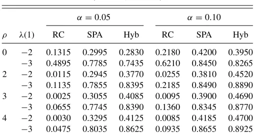
Table 3. Empirical power of tests of predictive abilities under DGP A (M=50, n=200)
α=0.05 α=0.10
ρ λ(1) RC SPA Hyb RC SPA Hyb
0 −2 0.1315 0.2995 0.2830 0.2180 0.4200 0.3950
−3 0.4895 0.7785 0.7435 0.6210 0.8450 0.8265 2 −2 0.0115 0.2945 0.3770 0.0255 0.3810 0.4520
−3 0.1135 0.7855 0.8395 0.2185 0.8490 0.8890 3 −2 0.0025 0.3055 0.4085 0.0095 0.3900 0.4690
−3 0.0655 0.7745 0.8390 0.1360 0.8345 0.8770 4 −2 0.0030 0.3295 0.4125 0.0085 0.4185 0.4700
−3 0.0475 0.8035 0.8625 0.0935 0.8655 0.8925
Table 4. Empirical power of tests of predictive abilities under DGP A (M=100, n=200)
α=0.05 α=0.10
ρ λ(1) RC SPA Hyb RC SPA Hyb
0 −2 0.0945 0.2675 0.2475 0.1805 0.3765 0.3535
−3 0.3945 0.7080 0.6755 0.5270 0.7885 0.7755 2 −2 0.0025 0.2315 0.3185 0.0115 0.3040 0.3830
−3 0.0620 0.7040 0.7750 0.1230 0.7710 0.8220 3 −2 0.0000 0.2345 0.3245 0.0030 0.3110 0.3810
−3 0.0350 0.7115 0.7865 0.0725 0.7770 0.8230 4 −2 0.0005 0.2385 0.3125 0.0035 0.3155 0.3615
−3 0.0190 0.7220 0.7875 0.0435 0.7925 0.8250
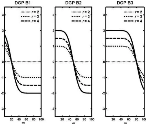
m=1, . . . , M,
DGP B1: λ(m)=r× {(−8m/M+1/5)−1/2},
DGP B2: λ(m)=r× {(−8m/M+2/5)−1/2}, and DGP B3: λ(m)=r× {(−8m/M+4/5)−1/2},
where is a standard normal distribution function and r is a positive constant running in an equal-spaced grid in [0,5].
This scheme is depicted in Figure 3. In DGP B1, only a small portion of methods perform better than the benchmark method, and in DGP B3, a large portion of methods perform better than the benchmark method. The general discussion of this article predicts that the hybrid test has relatively strong power against the alternatives under DGP B1, while it has relatively weak power against the alternatives under DGP B3.
Only the results for the cases DGP B1 and DGP B3 are shown in Figure 4 to save space. Under DGP B1, Hyb is shown to out-perform the other tests. However, it shows a slight reduction in power (relative to SPA) under DGP B3. This result suggests that
Figure 3. Three designs of λ (m) with M = 100. All the three designs represent different types of alternative hypotheses. In DGP B1, the forecasting methods withm=1 throughm=20 outperforms the benchmark method and in DGP B3, the forecasting methods withm= 1 throughm=80 outperforms the benchmark method.
Figure 4. Finite sample rejection probabilities for testing predictive ability for three tests at nominal size 5%: Reality Check (RC) test of White (2000), Superior Predictive Ability (SPA) test of Hansen (2005), and Hybrid (Hyb) test of this article against alternatives are depicted in Figure 3. The result shows that Hyb performs conspicuously better than SPA and RC under DGP B1 that is generally associated with low power for tests, and it performs slightly worse than SPA under DGP B3 that is generally associated with high power for tests. Hence the result illustrates the robustified power behavior of the hybrid approach.
as long as the simulation designs used so far are concerned, the power gain by adopting the hybrid approach can be considerable under certain alternatives while its cost as a reduction in power under the other alternatives is only marginal.
5. EMPIRICAL APPLICATION: REALITY CHECK REVISITED
5.1 Testing Framework and Data
The empirical section of White (2000) investigates forecasta-bility of excess returns using technical indicators. He demon-strated that unless the problem of data snooping is properly addressed, the best performing candidate forecasting method appears spuriously to perform better than the benchmark fore-cast based on a simple efficient market hypothesis. This sec-tion revisits his empirical study using recent S&P500 stock returns.
Similarly as in White (2000), this study considered 3654 forecasts using technical indicators and adopted MSPE defined as follows: form=1, . . . ,3654,
MSPE :MSPE(m)=E(Ym,T+1−Yˆm,T+1)2,
whereYT denotes the S&P500 return on dayT ,and ˆYT+1its one
day ahead forecast. (Given stock pricePt att, the stock return
is defined to beYt=(Pt−Pt−1)/Pt−1.) See White (2000) for
details about the construction of the forecasts.
S&P500 Stock Index closing prices were obtained from the Wharton Research Data Services (WRDS). The stock index returns data range from March 28, 2003, to July, 1, 2008. For
Song: Testing Predictive Ability and Power Robustification 295
Table 5. Bootstrapp-values for testing predictive ability in terms of MSPE. The numberqrepresents the tuning parameter that determines
the random block sizes in the stationary bootstrap. See Politis and Romano (1994) and White (2000) for details.
q RC SPA Hyb
Data snooping 0.10 0.1910 0.1598 0.0670 taken into account 0.25 0.2916 0.2736 0.0980 0.50 0.3378 0.3206 0.1250 Data snooping 0.10 0.0094 0.0094 0.0200 ignored 0.25 0.0188 0.0188 0.0390 0.50 0.0384 0.0384 0.0780
each forecast method, we obtain 187 one-day ahead forecasts from October 4, 2007, to July 1, 2008. The data used for the estimation of the forecast models begin from the stock index return on March 28, 2003, and the sample size for estimation is 1138. Hence the sample size for estimation is much larger than the sample used to produce forecasts, and it is expected that the normalized sum of the forecast error differences will be approximately normally distributed [see Clark and McCracken (2001) for details].
5.2 Results
The results are shown inTable 5. The number q in the ta-ble represents the tuning parameter that determines the random block sizes in the stationary bootstrap of Politis and Romano (1994) [see White (2000) for details]. Note that in White (2000),
q=0.5 was used.
Table 5 presents p-values for the tests with data snooping taken into account, and for the tests with data snooping ignored. When data snooping is ignored, all the tests spuriously reject the null hypothesis at 10%. (Note that the results of RC and SPA are identical, because there is only one candidate forecast when data snooping is ignored, and this forecast is not trimmed out by the truncation involved in SPA.) This attests to one of the main messages of White (2000) that without proper consid-eration of data snooping, the best performing candidate fore-casting method will appear to highly outperform the benchmark method.
Interestingly, thep-values from Hyb are conspicuously lower than those obtained from RC and SPA. For example, when
q=0.10, thep-values for RC and SPA are 0.1910 and 0.1598, respectively, but thep-value for Hyb is 0.0670. Hence the null hypothesis is rejected by Hyb while not by RC and SPA at 10% in this case. This illustrates the distinctive power be-havior of Hyb. Note that Hyb can outperform RC even when SPA does not outperform it. Such a case may arise when for all the m’s √ndˆ(m)/ωˆ(m) is greater than −√2 ln lnn with large probability, but for some m, √ndˆ(m)/ωˆ(m) still tends to take a fairly negative value relative to the critical valuecα
of RC.
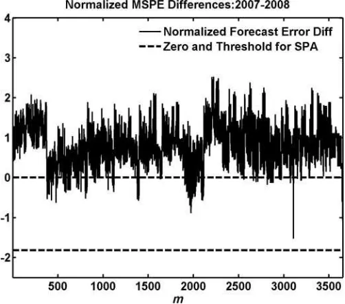
For example, see Figure 5 that plots the normalized MSPE differences, that is,√ndˆ(m)/ωˆ(m),form=1, . . . ,3654. It is interesting to see that no forecasting method is truncated by the truncation scheme of SPA. This is indicated by the fact that all the normalized forecast error differences are above the threshold
Figure 5. Normalized estimated mean forecast error differences in terms of MSPE [i.e.,√neˆ(m)/ωˆ(m)]. The threshold is−√2 ln lnn. The x-axis is the forecasting method indexmrunning from 1 to 3654. The forecast error differences lie above the threshold value (represented by the lower dashed line). This means that no forecast method was truncated by SPA in this case. Therefore, the difference between RC and SPA is solely due to the normalization by ˆω(m) in SPA. Even in this case, Hyb can still improve the power of the sup test through the power-enhancing effect from the complementary test.
value (lower dashed line). This perhaps explains similarp-values for RC and SPA. The difference between the results from RC and SPA is solely due to the fact that SPA involves normalization by ˆω(m) while RC does not. Even in this case, Hyb continues to counteract its power-reducing effect by coupling with the complementary test statistic.
6. CLOSING REMARKS
This article has shown that the one-sided sup tests of predic-tive ability can be severely asymptotically biased in a general setup. To alleviate this problem, this article proposes the ap-proach of hybrid tests where we couple the one-sided sup test with a symmetrized complementary test. Through simulations, it is shown that this approach yields a test with robust power behavior. The hybrid approach can be applied to numerous other tests of inequalities beyond predictive ability tests. The question of which modification or extension is suitable often depends on the context of application.
ACKNOWLEDGMENT
I thank Werner Ploberger and Frank Schorfheide for their valuable comments and advice. Part of this article began with a draft titled, “Testing Distributional Inequalities and Asymptotic Bias.” The comments of a Co-Editor, an Associate Editor, and a referee were valuable and helped improve the article substan-tially. I thank them for their comments.
[Received November 2009. Revised October 2011.]
REFERENCES
Amisano, G., and Giacomini, R. (2007), “Comparing Density Forecasts via Weighted Likelihood Ratio Tests,”Journal of Business and Economic Statis-tics, 25, 177–190. [288,290]
Andrews, D. W. K. (2011), “Similar-on-the-Boundary Tests for Moment In-equalities Exist but Have Poor Power,”CFDP1815.http://cowles.econ.yale. edu/P/cd/d18a/d1815.pdf[288]
Andrews, D. W. K., and Shi, X. (2011), “Inference Based on Conditional Mo-ment Inequalities,”CFDP1761R. http://cowles.econ.yale.edu/P/cd/d17b/ d1761-r.pdf[288]
Andrews, D. W. K., and Soares, G. (2010), “Inference for Parameters Defined by Moment Inequalities Using Generalized Moment Selection,”Econometrica, 78, 119–157. [288]
Bao, Y., Lee, T.-H., and Salto˘glu, B. (2007), “Comparing Density Forecast Models,”Journal of Forecasting, 26, 203–225. [288,289,290]
Bugni, F. (2010), “Bootstrap Inference in Partially Identified Models Defined by Moment Inequalities: Coverage of the Identified Set,”Econometrica, 78, 735–753. [288]
Canay, I. A. (2010), “EL Inference for Partially Identified Models: Large De-viations Optimality and Bootstrap Validity,”Journal of Econometrics, 156, 408–425. [288]
Christoffersen, P. F. (1998), “Evaluating Interval Forecasts,”International Eco-nomic Review, 39, 841–861. [288]
Clark, T. E., and McCracken, M. W. (2001), “Tests of Equal Forecast Accuracy and Encompassing for Nested Models,”Journal of Econometrics, 105, 85– 110. [295]
Diebold, F. X., Gunther, T. A., and Tay, A. S. (1998), “Evaluating Density Forecasts With Applications to Financial Risk Management,”International Economic Review, 39, 863–883. [288]
Diebold, F. X., Hahn, J., and Tay, A. S. (1999), “Multivariate Density Forecast Evaluation and Calibration in Financial Risk Management: High-Frequency
Returns on Foreign Exchange,”Review of Economics and Statistics, 81, 661–673. [288]
Diebold, F. X., and Mariano, R. S. (1995), “Comparing Predictive Accuracy,” Journal of Business and Economic Statistics, 13, 253–263. [288] Giacomini, R., and White, H. (2006), “Tests of Conditional Predictive Ability,”
Econometrica, 74, 1545–1578. [288,289,290]
Hansen, P. R. (2005), “Testing Superior Predictive Ability,”Journal of Business and Economic Statistics, 23, 365–379. [288,289,291,292,293]
Lee, S., Song, K., and Whang, Y.-J. (2011), “Testing Functional Inequalities,” Cemmap Working Paper, CWP12/11, Department of Economics, University College London. [290]
Linton, O., Maasoumi, E., and Whang, Y.-J. (2005), “Consistent Testing for Stochastic Dominance Under General Sampling Schemes,”Review of Eco-nomic Studies, 72, 735–765. [288,291]
Linton, O., Song, K., and Whang, Y.-J. (2010), “An Improved Bootstrap Test of Stochastic Dominance,” Journal of Econometrics, 154, 186– 202. [288]
Politis, D. N., and Romano, J. P. (1994), “The Stationary Bootstrap,”Journal of the American Statistical Association, 89, 1303–1313. [291,295]
Sullivan, R., Timmermann, A., and White, H. (1999), “Data Snooping, Technical Trading Rule Performance, and the Bootstrap,”Journal of Finance, 54, 1647–1692. [288]
Stinchcombe, M. B., and White, H. (1998), “Consistent Specification Test-ing When the Nuisance Parameters Present Only Under the Alternative,” Econometric Theory, 14, 295–325. [290]
West, K. D. (1996), “Asymptotic Inference About Predictive Ability,” Econo-metrica, 64, 1067–1084. [288]
West, K. D. (2006), “Forecast Evaluation,” inHandbook of Economic Fore-casting, Chapter 3, eds. G. Elliot, C. W. J. Granger, and A. Timmermann, North-Holland. [288]
White, H. (2000), “A Reality Check for Data Snooping,”Econometrica, 68, 1097–1126. [288,289,290,291,292,294,295]