Gender Disparities in High
Academic Achievement
Nicole M. Fortin
Philip Oreopoulos
Shelley Phipps
Fortin, Oreopoulos, and Phippsabstract
Using data from the “Monitoring the Future” surveys, this paper shows that from the 1980s to the 2000s, the mode of girls’ high school GPA distribution has shifted from “B” to “A,” essentially “leaving boys behind” as the mode of boys’ GPA distribution stayed at “B.” In a reweighted Oaxaca- Blinder decomposition of achievement at each GPA level, we fi nd that changes to gender differences in post- secondary expectations, in particular expectations for attending graduate or professional school, are the most important factors accounting for this trend after controlling for school ability and they occur as early as the eighth grade.
I. Introduction
Women now far outnumber men among recent college graduates in most industrialized countries (Vincent- Lancrin 2008). As Goldin, Katz, and Kuziemko
Nicole Fortin is professor of economics at the Vancouver School of Economics, University of British Columbia. Philip Oreopoulos is professor of economics at the University of Toronto. Shelley Phipps is pro-fessor of economics at Dalhousie University. All co- authors are Senior Research Fellows at the Canadian Institute for Advanced Research.
They would like to acknowledge Lori Timmins for her outstanding research assistance on this project. They would also like to thank Jerome Adda, Joseph Altonji, Marianne Bertrand, Russell Cooper, David Card, Steve Durlauf, Christian Dustmann, Andrea Ichino, Claudia Goldin, Larry Katz, John Kennan, Magne Mogstad, Mario Small, Uta Schonberg, Chris Taber, Thomas Lemieux, Glen Waddell, Ian Walker, Basif Zafar, and semi-nar participants at Bocconi University, Einaudi Institute for Economics and Finance, European University In-stitute, Federal Reserve Bank of New York, Harvard University, Norwegian School of Business and Econom-ics, Paris I, Sciences Po, University College London, University of Oregon, University of Wisconsin- Madison, Yale University, the CEA 2011, the CIFAR SIIWB Workshop, the NBER Summer Institute 2013, and SOLE 2012 for helpful comments on this and earlier versions of the manuscript. They thank ICPSR and MTF for allowing them to use the data, and the usual disclaimer applies. The authors are grateful for CIFAR’s fi nancial support. Fortin also acknowledges funding from SSHRC Grants #410- 2011- 0567. The data used in this article can be obtained beginning January 2016 through December 2019 from Nicole Fortin, Vancouver School of Economics, University of British Columbia, Vancouver, BC, V6T 1W1, nicole.fortin@ubc.ca.
[Submitted August 2012; accepted April 2014]
ISSN 0022- 166X E- ISSN 1548- 8004 © 2015 by the Board of Regents of the University of Wisconsin System This open access article is distributed under the terms of the CC- BY- NC- ND license (http://creativecommons.org/ licenses/by- nc- nd/3.0) and is freely available online at: http://jhr.uwpress.org
(2006) observe, the puzzle is: “Why have women overtaken men in terms of college completion instead of simply catching up to them?” The growing female dominance in educational attainment raises new questions about gender disparities arising through-out school ages.1 This paper addresses two questions: (1) Are boys and girls equally well prepared and focused on going to college? and (2) What accounts for the growing gender disparity in favor of girls obtaining high grades in secondary school?
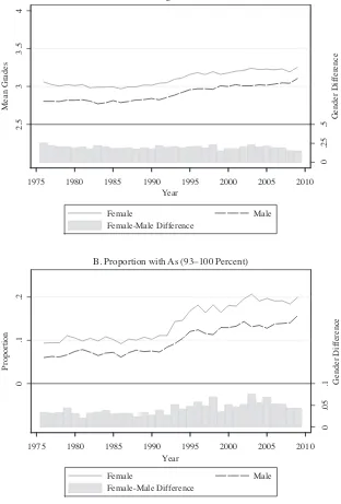
Our fi rst goal is to document changes in gender disparities in the academic perfor-mance of secondary school students (twelfth and eighth graders) over the last three de-cades using survey data from the “Monitoring the Future” (MTF) project.2 Girls have long obtained better grades in high school, on average, than boys. As shown in Figure 1a, the average gender gap in GPA among high school seniors (scaled out of four points) hovers steadily around 0.2 between 1976 and 2009.3 However, we
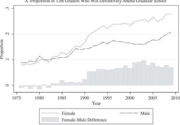
fi nd that over time an increasing proportion of students are earning A grades, arguably allowed by the progres-sive disaffection with “grading on a curve.”4 As shown in Figure 1b, the percentage of twelfth grade students reporting in the MTF that they earn As (93–100 percent) almost doubled, from 8.5 percent in the 1980s to 16.6 percent in the 2000s, and the difference between the proportion female and the proportion male in this category also doubled from 3.2 percent to 5.4 percent.5 From the 1990s to the 2000s, the female advantage in the proportion of eighth graders earning As also increased from 4.9 to 5.5 percentage points. Our second goal is to identify the relative importance of four sets of factors that changed differently by gender over time and that could account for this growing gender disparity in academic achievement. These include plans for the future, noncognitive skills, the family environment, and working while in school. The post- secondary aspirations and expecta-tions of high school students, as well as their choice of high school program (from voca-tional to academic) to enact these career plans, are the set of factors—called “plans for the future”—that changed the most over the last three decades. It is well known that returns to college have risen faster for men than for women over that period.6 Figure 2a shows that just the opposite happened to expectations about “defi nitively” attending a graduate or professional school after college. Among seniors, boys’ expectations about attending graduate school were slightly higher than girls’ from 1976 to 1983 but thereafter a gap in favor of girls began to emerge. In the early 1990s, following the computer revolution of the 1980s, the gap began to widen substantially, reaching nine percentage points before the Great Recession. Figure 2b presents the gender ratio among students who answer that
1. See for example, LoGerfo, Nichols, and Chaplin (2006); Machin and McNally (2005); Bertrand and Pan (2013). 2. To the best of our knowledge, Jacob and Wilder (2012) is the only other contemporaneous paper using the MTF to study educational expectations. They study the impact of these expectations on going to college. In Fortin, Oreopoulos, and Phipps (2013), we study the outcomes of tenth graders as well.
3. The gender gap in GPA from the MTF match (within standard errors) the numbers from the National Assessment of Educational Progress (NAEP) High School Transcript Study for 1990, 2000, 2005, and 2009, reported in Perkins et al. (2004), as well as the numbers reported in Cho (2007) for 1984 from the High School and Beyond survey.
0
.25
.5 Gender Dif
ference
2.5
3
3.5
4
Mean Grades
1975 1980 1985 1990 1995 2000 2005 2010
Year
Female Male
Female-Male Difference A. Average Grades
0
.05
.1 Gender Dif
ference
0
.1
.2
Proportion
1975 1980 1985 1990 1995 2000 2005 2010
Year
Female Male
Female-Male Difference
B. Proportion with As (93–100 Percent)
Figure 1
Self- Reported Grades of High School Seniors by Gender
Figure 2
Educational Expectations of High School Students
.3
.4
.5
.6
.7
Gender Ratio
1975 1980 1985 1990 1995 2000 2005 2010
Year Year
Among 12th Graders College Bound Among 8th Graders College Bound Among All 12th Graders
B. Gender Ratio Among Students Who Will Definitively Go to College
0
.1
.2
.3
Proportion
1975 1980 1985 1990 1995 2000 2005 2010
Female Male
Female-Male Difference
they “will defi nitively go to a four year college.” Among seniors, the gender ratio (female share) was around 50 percent up to the early 1980s, overshot the gender ratio in actual enrollment rates by a few percentage points in the 1990s, to stabilize around 57 percent in the 2000s; this corresponds to an excess 5 percent of girls given the 52 percent gender ratio among seniors.7 The gender ratio in expectations about attending a four- year college emerges as early as Grade 8, when it hovers around 55 percent.
Goldin and Katz (2002) have argued that the 1970s “Pill Revolution” was crucial in allowing young women to formulate plans for higher education without the fear of inter-ruptions for family reasons. We fi nd that in subsequent decades young women’s career plans increasingly involve professional and graduate schools and that clerical jobs have completely lost their appeal.8 Table 1 displays the dramatic changes in the vocational expectations of high school seniors (available only for a subsample). The percentage of girls thinking that they will be working at age 30 in a professional job requiring a post- graduate degree (doctoral or equivalent) climbed from 15.3 percent in the 1980s to 27.1 percent in the 2000s; for boys the change was from 13.5 to 16.4 percent. With the ad-vent of computerization and other offi ce technologies, there has been a substantial decline in labor market demand for clerical work matched by the decline in vocational expecta-tions: The percentage of girls expecting to work in a clerical job at age 30 has plummeted from 21 percent in the 1980s to less than 3 percent in the 2000s.9 This sharp decline is not matched by as great a decline in skilled and semiskilled work, craftsmanship, and protec-tive services as expected occupations for boys. Autor and Wasserman (2013) also argue that men have adapted less successfully than women to new labor market conditions. For our complete sample, our educational expectation variables include a full range of “plans for life after high school,” such as serving in the army, attending a vocational college, a two- year college, a four- year college, and aiming for graduate or professional school.
The data do not allow us to consider the effect from changes in teaching styles (Algan, Cahuc, and Shleifer 2010) or changes in teachers’ gender (Dee 2005) that have attracted recent attention. We do, however, include information on the types of high school program (academic, vocational, general, etc.) attended, which are associated with different GPA distributions.10 Following the wave of interest in the impact of non-cognitive traits, we account for smoking, alcohol binging, and school misbehavior.11 The other sets of factors that we consider are the family environment and working during school. Families with girls are, on average, larger (consistent with Angrist and
7. Appendix Figures A2a and A2b in Fortin, Oreopoulos. and Phipps (2013) illustrate how the see- saw pat-tern of the 1980s in Figure 2b arises from the changes in family planning methods 18 years earlier and the fact that boys are more likely than girls to repeat grades.
8. While we argue that changes in the labor market are likely the most important factors behind the changes in expectations, we cannot rule out the possible effect of changes in expectations about the likelihood of divorce. 9. Data from the Current Population Survey show that the actual proportion of young women (25–39 years old) employed in clerical work has dropped by 9 percent over the 35- year period while the proportion employed in professional occupations has increased by 9 percent (see Table A1 in Fortin, Oreopoulos, and Phipps 2013). 10. Similar information on the types of high school program (academic, general, vocational, etc.) in which students are enrolled is also asked in the NLS72 and NELS- 88, for example.
The Journal of Human Resources
Table 1
Vocational Expectations of Twelfth Graders by Gender
Years 1976–88 1989–99 2000–2009
Kind of Work Respondent Thinks Will Be Doing at Age 30 Boys Girls Boys Girls Boys Girls
Percentage in the labor forcea 99.9 93.2 99.7 97.7 99.6 98.3
Laborer, service worker, sales clerk 2.1 7.5 1.6 4.1 2.4 4.2
Skilled or semiskilled worker, Protective services (including military), farm owner
37.6 4.4 30.5 4.8 27.4 5.0
Clerical or offi ce worker 1.7 21.0 1.2 9.0 0.9 2.7
Owner of small business, sales representative, manager or administrator
17.3 14.4 17.9 13.5 16.9 12.8
Professional without doctoral degreeb 27.9 37.4 32.1 42.2 36.1 48.3 Professional with doctoral degree (or equivalent)c 13.5 15.3 16.7 26.4 16.4 27.1
Total in the labor force 100.0 100.0 100.0 100.0 100.0 100.0
Number of observations 18,369 19,343 11,667 12,560 9,242 10,396
Notes: Module 4 respondents were asked “What kind of work do you think that you will be doing when you are 30 years old? Mark the one that comes closest to what you expect to be doing.” Sixteen choices were possible including “Full- time homemaker” and “Don’t know” (6.7 percent of respondents). We regroup the 14 other choices into six categories for conciseness. More examples of specifi c jobs were given than reported.
aComputed as 100 minus the percentage of respondents choosing “Full- time homemaker or housewife.”
Evans 1998), have less- educated parents, more working mothers, and more fathers not living in the same household (see Dahl and Moretti 2008). These last two gender gaps in family characteristics are increasing over time. Finally, a decline in the labor force participation of boys during school, from 85 percent in the 1980s to 76 percent in the 2000s, has led to a closing of the gender gap in market work during high school. We focus on an analysis of changes over time in the distribution of GPA because gender differences in average GPA have not changed over the past 30 years while the gender ratio of students admitted to college, those with high GPA, has changed sub-stantially. As with most studies of changes in gender differentials, we construct coun-terfactual states of the world based on the observed responses (estimated coeffi cients) and respective endowments of males and females. We use the reweighted decomposi-tion methodology (Fortin, Lemieux, and Firpo 2011) to separate endowment effects from response effects. More precisely, we construct a counterfactual sample of boys re-weighted to have the same characteristics as girls. We then make the assumption that the distribution of unobservables, conditioning on observables, is independent of gender. Then differences between the educational responses from this counterfactual sample and those of girls refl ect true gender differences in educational responses (rather than misspecifi cation error because the underlying conditional expectation is nonlinear).
Our decomposition of the impact of educational expectations on GPA may only be in-terpreted as a direct effect if the distribution of unobservables conditional on observables is independent of gender. To explore whether changes in other factors, such as ability, returns to college, or fi nancial constraints, underlie changes in expectations, we use data from the MTF surveys on educational aspirations and subjective assessments of school ability. This allows us to consider indirect effects and to present bounds on the direct effects of educational expectations with and without these controls. With respect to the possibility of reverse causality, where changes to GPA distribution may affect education aspirations, we note that the sudden 1991 rise in the expectations of girls about pursuing a professional or graduate degree (Figure 2b) preceded and exceeded in size the 1993 marked rise in the proportion of girls obtaining As (Figure 1b). That being said, our anal-ysis uses selection on observables for identifying explanatory factors behind changes in educational aspirations rather than a quasi- experimental or experimental design.12
The rest of the paper is organized as follows. Section II introduces the MTF surveys and presents some descriptive statistics about gender disparities in academic achieve-ment and in the explanatory factors. Section III presents our empirical specifi cation and explains the reweighted decomposition methodology. Section IV presents the de-composition results and discusses their interpretation. Finally, Section V concludes.
II. Data and Descriptive Statistics
The data used are from the “Monitoring the Future” surveys that were conducted by University of Michigan’s Institute for Social Research mainly to monitor
substance abuse every year from 1976 onward for Grade 12 students and from 1991 onward for students in Grade 8.13 Given higher male dropout rates, our sample of twelfth graders is only 48 to 49 percent male. Thus, our sample of seniors likely com-prises a positively selected sample of boys, leading us to understate any gender gap favorable to girls by comparison to a wider sample of boys. It is thus useful to compare high school seniors with eighth graders, who remain subject to minimum age school leaving laws. We focus on the core sample, which is comprised of 10,000 to 16,000 observations per grade per year, and allows us to perform the breakdown by gender and GPA.14
Our dependent variable is the self- reported school grade that is elicited from the following question: “Core 20: Which of the following best describes your average grade so far in high school? D (69 or below), C– (70–72), C (73–76), C+ (77–79), B– (80–82), B (83–86), B+ (87–89), A– (90–92), A (93–100).”15 Obviously, grades from administrative data are preferable to self- reported grades because students with different characteristics may misreport their grades differently.16 But we fi nd that the self- reported grades from the MTF are very reliable.17 When we compare the aver-age grades of twelfth graders from the MTF to those of the High School Transcript Surveys (HSTS) of the NAEP (reported in Perkins et al. 2004) we fi nd that the gen-der differences, as well as the grade infl ation, do match within standard errors, even though the scales used are somewhat different.18 Note that this report
fi nds, as Goldin, Katz, and Kuziemko (2006) also reported, that girls are increasingly taking more challenging math and science courses. Card, Payne, and Sechel (2011) fi nd that the 10 percentage gender gap (female advantage) in university application rates of Ontario students is very strongly related to the fraction of students who take the academic versus applied mathematics test in Grade 9.
There are other questions in the MTF survey of seniors, asked before this one and directed at getting subjective assessments of school ability (Core 16) and intelligence (Core 17), which would allow students who are so inclined to boast about their abili-ties. The question on subjective school ability asks: “Core 16: Compared with others your age throughout the country how do you rate yourself on school ability? Far be-low average, bebe-low average, slightly bebe-low average, average, slightly above average,
13. Because of the focus on drug use, those who use illicit drugs as seniors are oversampled; we are careful to use the sample weights provided to remove any bias resulting from that oversampling. There exists a seldom accessed longitudinal component, which surveys a small subset of the students (Bachman et al. 2002). 14. Many more attitudes and behavioral questions are asked of students answering one of six modules, including a host of noncognitive variables, but they are asked only of a subset of students.
15. Following standard institutional practice, the self- reported grades in the nine categories are translated in the numbers: A (93–100) 4.0, A- (90–92) 3.7, B+ (87–89) 3.3, B (83–86) 3.0, B- (80–82) 2.7, C+ (77–79) 2.3, C (73–76) 2, C- (70–72) 1.7, D (69 or below) 1, where 2.3 and 2.7 and so on are the rounded versions of 2.333 and 2.666.
16. See Balsaa, Giuliano, and French (2011) on grade misreporting by alcohol binging students.
17. The wording of the question on self- reported grades in terms of an upward scale is similar to commonly used questions about self- reported income where individuals are asked to declare in which income bracket their income falls and may be less prone to error than simple declarative questions.
above average, far above average.”19 Boys and girls, on average, provide the same subjective ratings of their school ability but boys rate themselves more favorably on intelligence than do girls.20 We note that the raw correlation between subjective school ability and self- reported grades is only 58 percent among seniors.
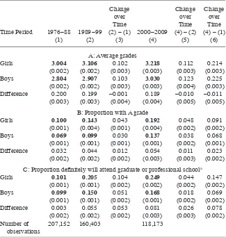
Table 2 begins by reporting a simple difference- in- difference analysis of the changes over time and by gender in self- reported grades and in expectations about attending graduate or professional school of twelfth graders. Like Figure 1, Panel A of Table 2 shows little change over time in the signifi cant female advantage of about 0.2 (on a four point scale) in average grades; if anything, boys have made small gains (about 0.01) in relative grades. Panel B shows that the stability in average grades masks a signifi cant increase in the female advantage in the proportion of students with the highest grades (A [93–100] students), which represents the pool of students that can be confi dent of being admitted to graduate school if they continue to succeed in their undergraduate studies. Our focus on the gender gap in top grades follows from the fi ndings of previous studies (Jacob 2002; Goldin, Katz, and Kuziemko 2006; Cho 2007; Conger and Long 2010) showing that the lower college admission rates of men can in large part be accounted for by their lower high school performance.21 However, better high school performance explains “how” more girls are admitted to college but not “why.”
As in Figure 2a, Panel C of Table 1 shows an even greater and signifi cant increase of the female advantage in expectations of attending professional or graduate school. Indeed, from the 1980s to 1990s, the proportion of women expecting to attend gradu-ate school more than doubled from 10 percent to 21 percent while the proportion of men increased only by half, from 10 percent to 15 percent. The fact that the increase in the gender differential in expectations to attend graduate school was more sizeable (5.3 percentage points) from the 1980s to the 1990s, when women’s progress in the la-bor market was sharpest, than from the 1990s to the 2000s (2.6 percentage points) are in line with our conjecture that gender differences in plans for the future fuel gender differences in high academic achievement. But we do not claim to have fi rm evidence on the causes of the changes in educational expectations.
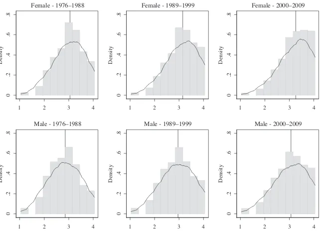
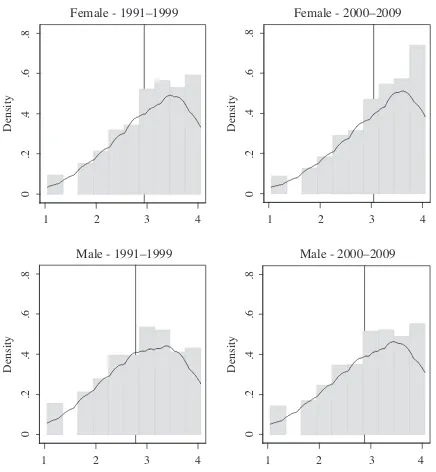
A more complete picture of changes in academic achievement is presented in Figure 3, which displays histograms corresponding to the actual data overlaid with a kernel density of the self- reported grades of girls and boys in twelfth grade. The fi gures clearly show a progressive disaffection over the past 35 years with “grading on a curve,” with the alternative “competency grading” gaining in importance.22 In the 1980s, the mode
19. As with the other categorical variables, we rescale this variable to be between 0 and 1 using the following formula: Category k = 1 – (n – k + 1)/(n+1), when k = n is highest category to be recoded into 1. This recoding presumes equal distance between the categories.
20. The question on intelligence asks on the same seven point scale: “Core 17: How intelligent do you think you are compared with others your age?” See Fortin, Oreopoulos, and Phipps (2013), Figures A3a and A3b. 21. The higher average grades of girls are at times equated with their higher average noncognitive abilities (Jacob 2002; Becker, Hubbard, and Murphy 2010). Alternatively, Cornwell, Mustard, and Van Parys (2013) argue that discrepancies between test scores and grades by gender are due to discrimination by teachers. If teachers discriminate on the basis of classroom behavior rather than pure gender preference, grades would incorporate some noncognitive abilities.
Table 2
Difference- and- Differences Estimates in Academic Performance and Plans for the Future - Twelfth Graders
Girls 3.004 3.106 0.102 3.218 0.112 0.214
(0.002) (0.002) (0.003) (0.003) (0.003) (0.003)
Boys 2.804 2.907 0.103 3.030 0.123 0.225
(0.002) (0.002) (0.003) (0.003) (0.004) (0.003)
Difference 0.200 0.199 –0.001 0.189 –0.010 –0.011
(0.003) (0.003) (0.004) (0.004) (0.005) (0.005)
B: Proportion with A grade
Girls 0.100 0.143 0.043 0.192 0.048 0.091
(0.001) (0.004) (0.001) (0.004) (0.002) (0.002)
Boys 0.069 0.099 0.030 0.137 0.038 0.068
(0.001) (0.001) (0.001) (0.001) (0.002) (0.001)
Difference 0.032 0.044 0.012 0.054 0.011 0.023
(0.002) (0.002) (0.002) (0.003) (0.003) (0.002)
C: Proportion defi nitely will attend graduate or professional schoola
Girls 0.101 0.205 0.104 0.249 0.044 0.147
(0.001) (0.001) (0.002) (0.002) (0.002) (0.002)
Boys 0.099 0.150 0.051 0.168 0.018 0.069
(0.001) (0.001) (0.002) (0.001) (0.002) (0.002)
Difference 0.003 0.055 0.053 0.081 0.026 0.078
(0.002) (0.002) (0.002) (0.003) (0.003) (0.002)
Number of observations
207,152 160,403 118,173
Notes: Self- reported grades in nine categories (D, C- , C, C+, B- , B, B+, A- , A) are translated into the numbers 1, 1.7, 2, 2.3, 2.7, 3, 3.3, 3.7, and 4 following standard institutional practice.
aThe numbers for other post- secondary choices are reported in Table 3.
and median of the grades distribution roughly coincided in the B range. By the 2000s, the mode of the girls’ grade distribution had moved from B to A, while the mode of the boys’ grade distribution stayed at B.23 This is what we call “leaving boys behind”; although the proportion of boys in the A range has increased over time, the gender gap in the proportion of students at the very top of the GPA distribution has increased.
Figure 4 reports the same data on eighth graders for two time periods, 1991–99 and 2000–2009. Here, the girls’ advantage appears even more dramatic.
One may wonder whether these distributional changes arise from increases in the mean grade pushing the upper tail against the upper boundary or from increases in the upper tail pulling the mean. With the fi rst hypothesis, the explanations behind the increases in mean grade remain unspecifi ed under the heading “grade infl ation.” We test this hypothesis by fi rst estimating an ordered probit of GPA levels for the three time periods and then using the estimated cutoffs of the second and third period to infl ate the predictions from a similar model estimated only on the fi rst period. The resulting predictions for the A and B+ levels are found to be below the observed ones, which tells us that this type of grade infl ation is not suffi cient to lead to the observed increases in the proportion of students getting the high grades.
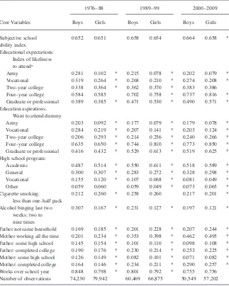
The means of selected explanatory variables for seniors are reported in Table 3 for each of the three time periods of interest.24 The fi rst row displays the students’ own evaluation of their school ability. It shows that despite having lower grades, boys rate
24. The statistics are computed on observations with no missing variables. This reduces the sample sizes by comparison with Table 2. Complete descriptive statistics for twelfth graders are presented in Table A2 of Fortin, Oreopoulos, and Phipps (2013). Descriptive statistics for eighth graders are available upon request.
Male and Female Densities of Self- Reported Grades Among Twelfth Graders
their own school ability higher than girls.25 Similar male overconfi dence has been reported among college students by Stinebricker and Stinebricker (2012) who fi nd that college- bound boys are less likely to succeed because of their overall lower perfor-mance.26
The variables capturing the plans for the future follow. Among twelfth graders, the fi rst question about post- secondary plans asks about expectations: “Core 21: How likely (defi nitively won’t, probably won’t, probably will, defi nitively will) is it that you will do each of the following things after high school? (a) attend a technical or vocational school, (b) serve in the armed forces, (c) graduate from a two- year college, (d) graduate from college (four- year program), (e) attend graduate or pro-fessional school after college?” A second question asks about aspirations: “Core 22: Suppose you could do just what you’d like and nothing stood in your way. How many
25. Girls in 1976–88 and boys in 2000–2009 have similar average GPA of 3.0 but the boys’ school ability index of 0.664 is signifi cantly greater than the girls’ 0.651.
26. Although grades by topic are not reported in the MTF, numerous studies (especially those using the Na-tional Education Longitudinal Study) show that boys continue to maintain an advantage in math test scores (but not in math grades), especially at the high end of the distribution. The boys’ overconfi dence may be built on these scores.
Figure 4
Male and Female Densities of Self- Reported Grades Among Eighth Graders
Table 3
Means of Selected Core Variables by Gender—Twelfth Graders
1976–88 1989–99 2000–2009
Core Variables Boys Girls Boys Girls Boys Girls
Subjective school ability index
0.652 0.651 0.658 0.654 0.664 0.658 *
Educational expectations: Index of likeliness to attenda
Army 0.281 0.102 * 0.215 0.078 * 0.202 0.079 *
Vocational 0.319 0.264 * 0.268 0.210 * 0.274 0.208 *
Two- year college 0.338 0.364 * 0.362 0.370 * 0.383 0.386
Four- year college 0.584 0.585 0.702 0.758 * 0.737 0.816 *
Graduate or professional 0.389 0.385 * 0.471 0.530 * 0.490 0.571 *
Education aspirations: Want to attend dummy
Army 0.203 0.092 * 0.177 0.079 * 0.179 0.078 *
Vocational 0.284 0.219 * 0.207 0.141 * 0.203 0.124 *
Two- year college 0.206 0.293 * 0.214 0.256 * 0.240 0.266 *
Four- year college 0.635 0.650 * 0.744 0.810 * 0.773 0.850 *
Graduate or professional 0.416 0.432 * 0.529 0.613 * 0.519 0.625 *
High school program:
Academic 0.487 0.514 * 0.550 0.611 * 0.518 0.589 *
General 0.300 0.307 * 0.283 0.272 * 0.328 0.298 *
Vocational 0.155 0.120 * 0.107 0.068 * 0.081 0.049 *
Other 0.059 0.060 0.059 0.049 * 0.073 0.065 *
Cigarette smoking: less than one- half pack
0.212 0.260 * 0.258 0.260 0.217 0.201 *
Alcohol binging last two weeks: two to nine times
0.307 0.167 * 0.231 0.127 * 0.197 0.121 *
Father not same household 0.169 0.185 * 0.201 0.228 * 0.207 0.244 *
Mother working all the time 0.201 0.234 * 0.353 0.398 * 0.462 0.495 *
Father: some high school 0.145 0.154 * 0.101 0.110 * 0.098 0.108 *
Father: completed college 0.190 0.176 * 0.230 0.214 * 0.253 0.225 *
Mother: some high school 0.126 0.149 * 0.082 0.101 * 0.071 0.082 *
Mother: completed college 0.164 0.146 * 0.234 0.211 * 0.290 0.257 *
Works over school year 0.848 0.798 * 0.801 0.792 * 0.755 0.756
Number of observations 74,230 79,942 60,469 66,875 50,549 57,202
Notes: Asterisk indicates statistically signifi cant gender difference at the 5 percent level. Means of other variables and other categories are reported in Fortin, Oreopoulos, and Phipps (2013).
of the following things would you WANT to do?” with the fi ve options above be-ing supplemented by “none of the above.” The expectations question raises issues of endogeneity with respect to GPA. Some high- ability students may have low expecta-tions of graduating from a four- year college because of their low GPA, rather than the other way around. The aspirations question attempts to circumvent that problem with the preamble if “nothing stood in your way.” Controlling for subjective school ability (Core 16 above) and aspirations (Core 22) is an attempt to alleviate concerns about cognitive dissonance. Among eighth graders, the issue of endogeneity of edu-cational expectations is presumably less severe as there is more time to adjust one’s level of effort.27 For these students, we control for two retrospective measures of school ability (grade retention and whether school was often hard) as well as school misbehavior.28
Table 3 shows that in the 1980s, although seniors of both genders had similar ex-pectations about graduating from college and attending graduate school, girls already had higher aspirations (close to two percentage points) than boys. By the 2000s, the expectations index for both college and graduate school was eight percentage points higher for girls than boys.29 Gender differences in aspirations for college and graduate school are respectively eight percentage points and eleven percentage points higher in favor of girls. Finally, 6 percent of boys versus 3 percent of girls have declared no post- secondary aspirations. Next, the types of high school programs show that the gap in favor of girls in the proportion of seniors enrolled in an academic program has grown. While about 3 percent more girls than boys were enrolled in an academic pro-gram in the 1980s, that proportion increased to 7 percent in the 2000s. Among eighth graders, already 4 percent more girls than boys report being enrolled in a college preparatory program although a large proportion of students (43 percent of both boys and girls) have not made clear choices yet.
Table 3 also presents some selected demographic characteristics. The high alcohol binging category shows that boys are still more likely than girls to report these risky behaviors. Girls tend to live in families that might appear less likely to foster high academic achievement. Four percent more girls than boys report not living in the same household as their father, 3 percent more girls than boys report that their mother works all the time, and about 3 percent more boys than girls report that their father or mother has completed college.30 The fi nal row shows that the gender gap in paid work participation has closed over time, although boys continue to work longer hours and get higher pay.
27. Among eighth graders, only the expectations questions are asked.
28. More precisely, responses to the grade retention question “Have you ever had to repeat a grade in school?” are available as a binary variable. The responses to the two questions: “Now thinking back over the past year in school, how often did you . . . fi nd the school work too hard to understand?” “ . . . get sent to the offi ce, or have to stay after school, because you misbehaved?” were coded on a fi ve point scale.
29. Comparing seniors in 1972 from the NLS72, in 1980 from the H&B, in 1992 from the NELS88, and in 2004 from the ELS2002, Ingels, Dalton, and LoGerfo (2008) also fi nd that in 2004 more girls than boys expected to pursue graduate studies, whereas it was the opposite in 1972.
III. Empirical Speci
fi
cation and Reweighted
Decomposition Methodology
Our empirical specifi cation is based on a behavioral threshold model of academic performance where educational goals, fashioned in elementary school and likely infl uenced by parental desires, play a prominent role in determining, given a level of aptitude, an individual’s choice of optimal GPA.31 This follows an emerg-ing consensus in the psychology literature that students form reliable perceptions of their academic competency around fi fth grade (Herbert and Stipek 2005) and already can form some expectations about going to college.32 Indeed, decisions to enroll in a college preparatory high school program, to move to a neighborhood with a better high school, and to apply to a magnet school have to be made early in a student’s life. Under the assumption that effort is costly, the student’s optimal choice of GPA will be the minimum of the range that opens the door to the education level needed to fulfi ll her/his vocational goals. Students motivated toward professional or medical careers will come to understand they need to aim for As. Those thinking about white- collar occupations, such as fi nancial analyst, will need a bachelor’s degree and can aim for Bs; those expecting jobs that require fewer credentials may instead aim for Cs.
The changes over time in the shape in the distribution of GPA levels from a bell shape to a staircase shape (shown in Figures 3 and 4) are consistent with a threshold model in the presence of changes in career expectations, especially for girls. The less pronounced change in shape among boys would be consistent with more convex costs of effort, possibly associated with higher psychic or social costs of being seen as working hard.33 This type of threshold model helps rationalize the relative underper-formance of boys as the consequence of career choices that require lower levels of educational attainment. We do not exclude the possibility that some students revise their plans, but because we do not have access to the MTF longitudinal data, we can-not explore this avenue.34 Another attractive strategy could have used changes over time in local labor market opportunities by gender as an instrument to predict exog-enous variations in gender specifi c student expectations. Here again, we lack informa-tion about geographical locainforma-tion to exploit cross- secinforma-tional changes in labor market or other exogenous changes.
In this study of gender gaps in academic achievement, we simply seek to identify how student characteristics map into the distribution of GPAs differently by gender. We are primarily interested in how changes over time in these determinants help ac-count for changes over time in gender differentials in academic achievement. For each of the three time periods, we estimate the following academic achievement equation,
(1) Prob[Gi= c]= hg c(S
i,Ai,Li;Xi,Xi p),
c=1, …, 9,
31. The underlying model is exposited in Appendix B of Fortin, Oreopoulos, and Phipps (2013). 32. This is consistent with the high school tracking taking place in many European countries around the ages of ten and 11 (for example, Dustmann 2004).
where Gi is the student’s GPA, Si denotes the student’s educational goals, and Ai de-notes the student’ academic aptitude. We combine the high school program, the schooling expectations, and aspirations to measure Si. The student’s school aptitude, Ai, is proxied using the subjective measure of school ability (introduced in Section II) available for twelfth grade students.35 For eighth grade students, we measure aptitude by how often he or she found school “too hard” in the last year, in addition to a mea-sure of past grade retention. We include an indirect meamea-sure of effort, following the tradition in labor economics of deriving nonmarket time, here study time, as the dif-ference between total time (T) and labor market time (Li): Ei = T – Li. To explore the impact of noncognitive skills, we include measures of cigarette smoking and alcohol binging, which may relate to time impatience, and a measure of school misbehavior for eighth graders. Exogenous characteristics of student Xi are included, including race and living in an SMSA, as well as an extended set of family characteristics, Xi
p,
thought to be predetermined variables.36
We estimate a different linear probability model by gender for each level of GPA, which carries some advantages and disadvantages. The advantages of using a linear probability model are that we do not have to rely on the assumptions of normality of residuals. By comparison with an ordered probit model, this model allows the educa-tional responses to be different by level of GPA. Given that the detailed decomposi-tion of the gender differentials requires linear educadecomposi-tional responses, this estimadecomposi-tion procedure gives us coeffi cients that can readily be used.37
We use an extension (Fortin, Lemieux, and Firpo 2011) to the standard Oaxaca- Blinder (OB) decomposition that allows us to analyze the impact of gender differences in the educational response functions. We now give a short summary of the formulas behind this modifi ed decomposition. With the standard OB decomposition, the re-searcher seeks to determine what portion of the gender gap in grades is attributable or “explained” by differences in the characteristics of boys and girls and what portion re-mains “unexplained.” Here, owing to reweighting, we can argue that the “unexplained” part corresponds to gender differences in the structural function hg
c(S
i,Ai,Li;Xi,Xi p) of Equation 1. In the detailed decomposition, we can apportion parts of the aggregate de-composition to particular explanatory factors and responses to determine their relative importance.
Assuming that grades (G) can be modeled as a linear (in the parameters) function of characteristics (X) that is different for girls (F = 1) and boys (F = 0).
E(G |X,F =1) =E(X |F =1)1 and E(G| X,F =0) =E(X |F =0)0, under the zero conditional mean assumption, E(|X,F)=0. The classic OB coun-terfactual, E(GOB)=
E(X |F =1)0, asks “What would boys’ grades be if they had the same characteristics as girls?” using the coeffi cients estimated on the sample of
35. Educational aspirations and subjective school ability measures are available only for the twelfth graders. Clearly, lagged measures would have been preferred.
36. These family environment characteristics include living in the same household as the father, the mother, and siblings (separate questions), the number of siblings, whether the mother had a paid job while growing up (not at all, some of the time, most of the time, all the time), and the level of education (six levels) of the father and of the mother.
boys. As shown in Fortin, Lemieux, and Firpo (2011), with reweighting we can con-struct a counterfactual that more precisely isolates the educational responses. This counterfactual uses the coeffi cients estimated using the grades outcomes of boys but the characteristics of the sample of boys reweighted to be like girls.
More precisely, we reweight the sample of boys so that the distribution of their characteristics (X) is similar to that of girls using the following reweighting function
⌿(X)=[(Prob(X |F =1)) / (Prob(X |F =0))]
=[(Prob(F =1 | X)) / (Prob(F =0 | X))]⋅[Prob(F =0) /Prob(F =1)].38 The counterfactual coeffi cients 1o are estimated on the sample of boys reweighted
to look like girls’ {X0,⌿(X0)}. The difference (1− o
1) re
fl ects the true gender gap in educational responses, and the counterfactual means are computed as:
X0
1=⌺{i:F =0} ⌿(X
i)⋅ Xi. The reweighted decomposition uses the predicted grades, (X0|F =1)o
1 , from the reweighted sample as counterfactuals,
⌬O,R=E(X |F =1)1−E(X0|F =1)o
1+
E(X0|F =1)o
1−
E(X |F =0)0
= ⌬E,R + ⌬
X,R
to obtain an aggregate decomposition as the sum of an educational response effect,
⌬E,R, and a composition effect, ⌬X,R. Inasmuch as grade dummies can be averaged out, this decomposition relies on the additional assumptions of common support and ignor-ability (F ⊥ |X); that is conditioning of observables, unobservables are assumed to be the same across gender.39
Each term of the reweighted decomposition can be further broken down into the “pure” effect and a residual term. The composition effect, ⌬X,R, is written as the sum of a pure composition effect, ⌬X,p, and a specifi cation error, ⌬X,e,
⌬X,R
= E(X0|F =1)1o−E(X |F =0)0+E(X0|F =1)0−E(X0|F =1)0
=[E(X0|F =1)−E(X |F =0)]0+E(X0|F =1)(o1−0)
= ⌬X,p + ⌬X,e.
Similarly, the educational response term, ⌬E,R, can be written as the sum of a pure re-sponse effect ⌬E,p plus a reweighting error ⌬E,e,
⌬E,R
=E(X |F =1)1−E(X0|F =1)]1o−E(X |F =1)1o+E(X |F =1)1o =E(X |F =1)(1−1o) + [E
(
X |F =1)
−E(X0|F =1)]1o
= ⌬E,p + ⌬E,e.
38. The second equation makes use of Bayes’ Law to allow the computation Ψ(X) in the case of continuous X variables. See DiNardo, Fortin, and Lemieux (1996) for details.
The specifi cation error ⌬X,e= E(X0|F =1)(o
1−
0) corresponds to the difference in
the composition effects estimated by reweighting and by using simple regressions, where E(X0|F =1) is the mean of the reweighted sample; it captures the departures
from nonlinearity. The reweighting error ⌬E,e
=[E(X |F =1)−E(X0|F =1)]1o goes to zero in a large sample.
Because of the linearity of these expressions, the detailed decomposition or the ap-portionment of the composition and educational response effects to each explanatory variable is straightforward. In practice, this detailed reweighted decomposition can be obtained by running two decompositions: OB(1) with the sample of girls (F = 1) and the reweighted sample of boys looking like girls to get the pure educational response effect; and OB(2) with the sample of boys (F = 0) and the reweighted sample of boys looking like girls to get the pure composition effect.
IV. Empirical Results
Before going on to the decomposition results, it is useful to show which of our explanatory variables are more signifi cant in explaining a cross- section in grade outcomes and how these relationships differ by gender. To conserve space, we report selected estimated coeffi cients only for seniors in the 2000s and only for the two GPA levels where the gender achievement gaps are largest, that is, for the A and C+ grades, and only for girls and boys, and not for the reweighted sample of boys, which are used in the decompositions.40
A. Determinants of Top and Below Average GPA
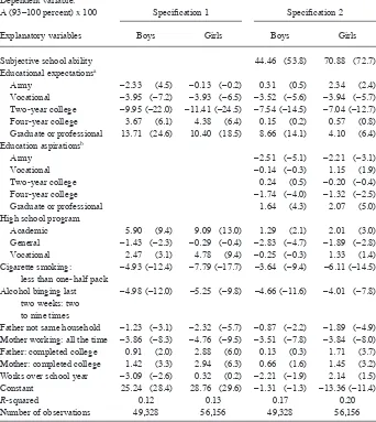
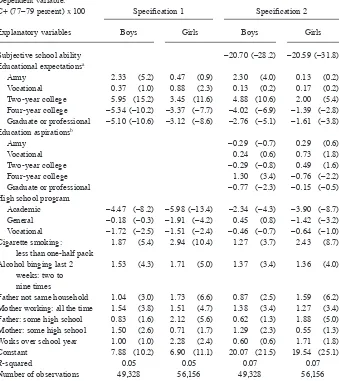
Tables 4a and 4b report the estimated coeffi cients of the explanatory variables listed in Table 3 along with t- statistics. In Table 4a, the dependent variable is equal to 100 if the student gets an A and 0 otherwise so that the coeffi cients indicate the added probability of getting an A associated with the explanatory variables. In Table 4b, we estimate the covariates of getting exactly a C+. Specifi cation 1 includes educational expectations under the assumption that students take their abilities and other limita-tions into account when formulating their expectalimita-tions. Specifi cation 2 explores the consequences of this assumption by explicitly controlling for subjective school abil-ity and for educational aspirations formed without possible limitations resulting from ability or other constraints.41 When we control for student ability and student aspira-tions, the explanatory power of expectations is reduced; this is indicative of potential endogeneity biases that we can control for only to some extent. Yet educational expec-tations remain among the most signifi cant explanatory variables. In Table 4a, wanting and expecting to attend graduate school, especially among boys, is associated with a higher probability, in the four to fourteen percentage point range of getting an A. Conversely, expecting to go to a two- year college shows a negative association, in the
40. The coeffi cients estimated on the reweighted sample are available upon request; they are generally close to the ones estimated on the sample of boys.
–7 to –11 percentage point range with getting an A. Expecting to go to a four- year col-lege is so widespread that it has little explanatory power. In Table 4b, consistent with our threshold model, expecting to go to a two- year college is associated with a higher probability, in the two to six percentage point range of getting a C+ , again especially for boys.42 The types of high school program, thought to be part of a student’s plans for the future, show similarly strong associations with these GPA levels and signifi cant differences across genders. Girls in academic high school programs are more likely to get an A and less likely to get a C+ than boys.
As in Balsaa, Guiliano, and French (2011), alcohol binging is associated with a sig-nifi cantly lower probability of getting an A, about –4 percentage points, and a higher probability of getting a C+, about one to four percentage points. Similar effects are found for smoking variables, in the –3 to –6 percentage point range for getting an A and the plus two percentage point range for a C+. We view these correlations as symptomatic of time impatience or caring less about the future. Focusing on family background variables, we fi nd that controlling for school ability (going from Speci-fi cation 1 to 2) substantially reduces the impact of parental education on students’ probabilities of getting an A or a C+ although that association remains signifi cant for girls.43 To the extent that parental education is capturing the family socioeconomic status, these results are consistent with past research (for example, Cameron and Heckman 2001, Reynolds and Pemberton 2001), showing that the biggest infl uence of parental resources on the children’s education operates through academic perfor-mance. Other important family infl uences, more impervious to the addition of subjec-tive school ability, are the actual presence of parents in the household. The father not living in the same household and the mother working have signifi cant effects (about –1 to –4 percentage points) on the probability of getting an A, and positive effects on the probability of getting a C+ (about one to two percentage points). Interestingly, the effect of the absent father is somewhat greater for girls and that of the mother working is somewhat greater for boys. Consistent with Buchmann and DiPrete (2006), we fi nd that these effects have increased from the 1980s to the 2000s. In comparison to the above regressors, the effects of the variables related to working during school are gen-erally less signifi cant and show some of the nonlinear patterns found in the literature.
B. Tabular Decomposition Results for Selected GPA Levels
In Table 5, we present the detailed decompositions for the 2000–2009 time period, for these two GPA levels for seniors and for the eighth grade students.44 The results for
42. This interesting new fi nding would be masked if the dependent variable was getting at least C+. In this case, expecting to go to a four- year college dominates.
43. When the specifi cation excludes educational expectations (see Fortin, Oreopoulos, and Phipps 2013, Specifi cation 3 in Table A3), the coeffi cients of parental education are larger.
44. The list of variables available for eighth graders is the following: dummies for race (white/non- white), SMSA, ever held back, smoked cigarettes per day (4), alcohol binging within last two weeks (4), sibling not same household, father not same household, mother not same household, mother working (3), father’s educa-tion (7), mother’s educaeduca-tion (7), worked during school, average hours of work (6), average earnings (7), type of high school program (4), indexes for school misbehavior last year, school too hard last year, educational expectations (army, vocational, go to college, complete 4- year college). So the main differences with
Table 4a
Selected Coeffi cients of LPM on Specifi c Grades - Twelfth Graders 2000–2009
Dependent variable:
A (93–100 percent) х 100 Specifi cation 1 Specifi cation 2
Explanatory variables Boys Girls Boys Girls
Subjective school ability 44.46 (53.8) 70.88 (72.7)
Educational expectationsa
Army –2.33 (4.5) –0.13 (–0.2) 0.31 (0.5) 2.34 (2.4)
Vocational –3.95 (–7.2) –3.93 (–6.5) –3.52 (–5.6) –3.94 (–5.7)
Two- year college –9.95 (–22.0) –11.41 (–24.5) –7.54 (–14.5) –7.04 (–12.7)
Four- year college 3.67 (6.1) 4.38 (6.4) 0.15 (0.2) 0.57 (0.8)
Graduate or professional 13.71 (24.6) 10.40 (18.5) 8.66 (14.1) 4.10 (6.4) Education aspirationsb
Army –2.51 (–5.1) –2.21 (–3.1)
Vocational –0.14 (–0.3) 1.15 (1.9)
Two- year college 0.24 (0.5) –0.20 (–0.4)
Four- year college –1.74 (–4.0) –1.32 (–2.5)
Graduate or professional 1.64 (4.3) 2.07 (5.0)
High school program
Academic 5.90 (9.4) 9.09 (13.0) 1.29 (2.1) 2.01 (3.0)
General –1.43 (–2.3) –0.29 (–0.4) –2.83 (–4.7) –1.89 (–2.8)
Vocational 2.47 (3.1) 4.78 (9.4) –0.25 (–0.3) 1.33 (1.4)
Cigarette smoking: less than one- half pack
–4.93 (–12.4) –7.79 (–17.7) –3.64 (–9.4) –6.11 (–14.5)
Alcohol binging last two weeks: two to nine times
–4.98 (–12.0) –5.25 (–9.8) –4.66 (–11.6) –4.01 (–7.8)
Father not same household –1.23 (–3.1) –2.32 (–5.7) –0.87 (–2.2) –1.89 (–4.9) Mother working: all the time –3.86 (–8.3) –4.76 (–9.5) –3.51 (–7.8) –3.84 (–8.0) Father: completed college 0.91 (2.0) 2.88 (6.0) 0.13 (0.3) 1.71 (3.7) Mother: completed college 1.42 (3.3) 2.94 (6.3) 0.66 (1.6) 1.45 (3.2) Works over school year –3.09 (–2.6) 0.32 (0.2) –2.21 (–1.9) 2.14 (1.5)
Constant 25.24 (28.4) 28.76 (29.6) –1.31 (–1.3) –13.36 (–11.4)
R- squared 0.12 0.13 0.17 0.20
Number of observations 49,328 56,156 49,328 56,156
Notes: Dependent variable is set to 100 if the student has a GPA of 4, and to 0 otherwise. T- statistics are in paren-theses. The base group for Alcohol binging and Cigarette smoking is none, Mother working is not working, Father’s and Mother’s education is high school, for High school program is other. The coeffi cients of the other variables and categories included in the regression are reported in Fortin, Oreopoulos, and Phipps (2013).
aIndex of educational expectations constructed from the four categories: defi nitively won’t, probably won’t,
prob-ably will, defi nitively will.
Table 4b
Selected Coeffi cients of LPM on Specifi c Grades - Twelfth Graders 2000–2009
Dependent variable:
C+ (77–79 percent) х 100 Specifi cation 1 Specifi cation 2
Explanatory variables Boys Girls Boys Girls
Subjective school ability –20.70 (–28.2) –20.59 (–31.8)
Educational expectationsa
Army 2.33 (5.2) 0.47 (0.9) 2.30 (4.0) 0.13 (0.2)
Vocational 0.37 (1.0) 0.88 (2.3) 0.13 (0.2) 0.17 (0.2)
Two- year college 5.95 (15.2) 3.45 (11.6) 4.88 (10.6) 2.00 (5.4) Four- year college –5.34 (–10.2) –3.37 (–7.7) –4.02 (–6.9) –1.39 (–2.8) Graduate or professional –5.10 (–10.6) –3.12 (–8.6) –2.76 (–5.1) –1.61 (–3.8) Education aspirationsb
Army –0.29 (–0.7) 0.29 (0.6)
Vocational 0.24 (0.6) 0.73 (1.8)
Two- year college –0.29 (–0.8) 0.49 (1.6)
Four- year college 1.30 (3.4) –0.76 (–2.2)
Graduate or professional –0.77 (–2.3) –0.15 (–0.5)
High school program
Academic –4.47 (–8.2) –5.98 (–13.4) –2.34 (–4.3) –3.90 (–8.7)
General –0.18 (–0.3) –1.91 (–4.2) 0.45 (0.8) –1.42 (–3.2)
Vocational –1.72 (–2.5) –1.51 (–2.4) –0.46 (–0.7) –0.64 (–1.0)
Cigarette smoking: less than one- half pack
1.87 (5.4) 2.94 (10.4) 1.27 (3.7) 2.43 (8.7)
Alcohol binging last 2 weeks: two to nine times
1.53 (4.3) 1.71 (5.0) 1.37 (3.4) 1.36 (4.0)
Father not same household 1.04 (3.0) 1.73 (6.6) 0.87 (2.5) 1.59 (6.2) Mother working: all the time 1.54 (3.8) 1.51 (4.7) 1.38 (3.4) 1.27 (3.4) Father: some high school 0.83 (1.6) 2.12 (5.6) 0.62 (1.3) 1.88 (5.0) Mother: some high school 1.50 (2.6) 0.71 (1.7) 1.29 (2.3) 0.55 (1.3)
Works over school year 1.00 (1.0) 2.28 (2.4) 0.60 (0.6) 1.71 (1.8)
Constant 7.88 (10.2) 6.90 (11.1) 20.07 (21.5) 19.54 (25.1)
R- squared 0.05 0.05 0.07 0.07
Number of observations 49,328 56,156 49,328 56,156
Notes: Dependent variable is set to 100 if the student has a GPA of 2.3, and to 0 otherwise. T- statistics are in paren-theses. The base group for Alcohol binging and Cigarette smoking is none, Mother working is not working, Father’s and Mother’s education is high school, for High school program is other. The coeffi cients of the other variables and categories included in the regression are reported in Fortin, Oreopoulos, and Phipps (2013).
aIndex of educational expectations constructed from the four categories: defi nitively won’t, probably won’t,
prob-ably will, defi nitively will.
The Journal of Human Resources
Table 5
Detailed Decomposition Results - Percentage Female/Male Difference for Selected GPA Levels
2000–2009 Twelfth Graders: Specifi cation 1 Twelfth Graders: Specifi cation 2 Eighth Graders
A (93–100) C+ (77–79) A (93–100) C+ (77–79) A (93–100) C+ (77–79)
Total differential 6.06 (0.007) –3.15 (0.005) 6.06 (0.007) –3.15 (0.005) 5.96 (0.007) –1.48 (0.005)
Composition effects
Fortin, Oreopoulos, and Phipps
571
Own school ability –0.09 (0.001) 0.01 (0.000) –0.10 (0.002) 0.14 (0.002) Educational expectations –0.12 (0.002) 0.15 (0.002) 1.08 (0.021) –1.33 (0.016) –0.21 (0.002) 0.10 (0.002) High school program 2.65 (0.028) –0.91 (0.020) 1.41 (0.027) –1.50 (0.020) 1.53 (0.008) –0.07 (0.006) Smoking, binging –0.47 (0.005) 0.34 (0.003) –0.33 (0.005) 0.32 (0.003) –0.04 (0.004) 0.35 (0.003) Race, SMSA –1.41 (0.013) –0.49 (0.009) –1.51 (0.013) –0.51 (0.009) –0.69 (0.013) –0.38 (0.009) Family background 1.59 (0.027) 0.31 (0.019) 1.09 (0.025) 0.71 (0.019) 1.54 (0.021) 0.73 (0.015) Work 1.59 (0.013) 0.30 (0.009) 1.62 (0.012) 0.09 (0.009) 0.46 (0.006) –0.04 (0.004) Constant –0.24 (0.043) –1.64 (0.030) 1.54 (0.045) –0.27 (0.034) 0.57 (0.021) –0.91 (0.020) Reweighting error 0.08 (0.003) –0.10 (0.001) 0.28 (0.003) –0.19 (0.001) 0.50 (0.003) –0.21 (0.001)
the earlier periods are reported in Fortin, Oreopoulos, and Phipps (2013) Appendix Tables A4 and A5. With regard to change over time in the aggregate decomposition for twelfth graders, most notable is the fact that the portions attributable to composition effects—the “explained” part—increased over the three time periods, especially at the top of the grade distribution.45 Averaging over all GPA levels, the “explained” part grew from a mere 10 percent of the total gender differential in the 1980s to 32 percent in the 1990s and to 37 percent in the 2000s. As we argue below, the larger increase from the 1980s to 1990s can be attributed to larger increases in the gender differential in educational expectations during that period.
We begin by discussing the composition effects in the upper panel of Table 5. Be-cause the female/male difference in school aptitude is negative, the effects of subjec-tive school ability for seniors, and of the two retrospecsubjec-tive measures of aptitude for eighth graders, go in the wrong direction: Their coeffi cients are positive for top grades and negative for mediocre grades. This reduces part of the gender differentials, nega-tive for top grades and posinega-tive for mediocre grades, accounted for by the explanatory variables. For example, in Table 5, see the reduction in “Total Explained” going from Specifi cation 1 to Specifi cation 2.46 We also note that race, living in a standard met-ropolitan statistical area (SMSA), and family background variables are other sets of “contrarian” or “swimming upstream” variables: These variables work to the advan-tage of boys (because there are more Black girls, more girls with absent father, etc.) and reduce the percentage of girls with top grades and of boys with mediocre grades. That is, if girls were as confi dent as boys about their school ability, if they lived in similar families, if there were as few Black girls living in SMSAs as boys, the girls’ grades would be even higher. In the 2000s, there would be from 0.6 to 0.9 percent more girls than boys earning As. Although minor, it is still interesting to fi nd that some high- achieving girls are “swimming upstream.”
Our major result is that educational expectations are the most important factor ac-counting for gender differentials in academic achievement. Table 5 shows that for seniors with A grades, gender differences in expectations account for 2.03 out of 2.44 percentage points of the “explained” by gender differences in characteristics (in Specifi cation 1) in the 2000s. This is up from 1.13 in the 1990s and from 0.23 in the 1980s.47 For the C+ grades, the numbers are –1.19 out of –1.22 percentage points of the “explained” in the 2000s, up from –0.66 in the 1990s and from –0.08 in the 1980s. As noted above, controlling for subjective school ability (Specifi cation 2) reduces the absolute magnitude of the gender differentials accounted for by expectations but not the portion explained. From the 1980s to the 2000s, the role of educational expecta-tions has gone from being virtually negligible to accounting for almost all gender differentials in these GPA levels.
For eighth graders, we fi nd similarly impressive results in the accounting power of expectations: For the A grades, the part explained by expectations is 1.53 out of
45. As illustrated in Figure 5 of Fortin, Oreopoulos, and Phipps (2013).
46. This effect is similar to the gender differences in educational attainment on the gender pay gap. In recent years, gender differences in education reduce the explained part of the gender pay gap. In the 2000s, the Total Explained corresponds to more than 40 percent of the gender achievement gap in Specifi cation 1 but only 17 percent in Specifi cation 2.
2.21 “Total Explained” in the 2000s, up from 1.07 in the 1990s. Overall, these results convey the same message as the one suggested by Table 2: That here, even after con-trolling for a host of other factors, gender differences in educational expectations (and changes therein) account for the largest share (and the most salient changes over time) in the gender differentials.
Noncognitive skills are another set of variables that has consistent explanatory power across all specifi cations for why girls have higher grades than boys. They are measured by smoking and alcohol binging among seniors and with the addition of school mis-behavior among eighthgraders. For top grades, they account for 0.49 to 0.56, and for 1.26 of the gender gap, among seniors and eighth graders, respectively. For mediocre grades, the numbers are large only for eighth graders. Among eighth graders, expecta-tions and noncognitive skills account for similarly large shares of the gender gap for top and mediocre grades. We fi nd that gender differences in noncognitive skills are the second most important factor to account for “explained” gender differences in academic achievement.48
Finally, we consider the contribution of changes in gender differences in educational responses presented in the bottom panel of Table 5, noting that the interpretation of these differences crucially depends on the omitted category in each case. The most important difference is linked to the type of high school program attended, where the omitted category is “other (not specifi ed) high school.” As we saw in previous tables, not only are girls increasingly attending college preparatory high school but they are benefi ting more (in terms of grades) from it than boys. This differential educational response adds to the total effect of “plans for the future” factors in accounting for gender differences in academic achievement.
The effects of gender differences in educational responses associated with family background is more diffi cult to interpret because departures from the omitted category (families with father present, mother present, one sibling, mother not working, both parents with high school education) are a more complex affair and the results are sen-sitive to which number of siblings is the omitted category (especially in the 1990s).49 Nevertheless, they indicate that family background generally bolsters the response of high- achieving girls by comparison with boys. A similar effect seems to apply to “work during school,” where the omitted categories are not working, zero hours of work, and zero wages.50 Working during school seems to act as a complement rather than a distraction for high- achieving girls.
C. Graphical Detailed Decomposition Results for all GPA Levels and Time Periods
Figure 5 for twelfth graders and Figure 6 for eighth graders display the results of the detailed decomposition for each GPA level for each category of factors. The lines trace the magnitude of the gender gap: Positive numbers indicate a larger value for females, negative numbers indicate a larger value for males. The numbers behind the
48. However, we fi nd some evidence that these effects are decreasing over time, at least for twelfth graders. 49. Such sensitivity is not surprising, given that even using an instrumental variable strategy that exploits exogenous variation in family size, Conley and Glauber (2006) fi nd a strong effect of sibship size on second- born boys’ grade retention but no effect on fi rst- born boys.
line graphs in Figure 5 show that the female advantage in the percentage of seniors getting As increases from 3.7 percentage points in the 1980s to 4.7 points in the 1990s to 6.1 points in the 2000s.51 At the same time, the male advantage in the C+ grade de-creases from 4.4 percentage points in the 1980s to 3.9 points in the 1990s to 3.2 points in the 2000s. Thus, for seniors, the changes in gender differentials to be accounted for correspond to 38 percent (2.3 percentage points) of the differential in top grades in the 2000s and to 40 percent (1.3 percentage points) for mediocre grades. The bars for each GPA levels are divided into two, the darker one capturing the composition effects of the factor of interest and the lighter the educational response effects to this factor. In
51. See Tables 5, A4, and A5. These numbers are a bit different from the ones reported in Table 1, Panel B, Row 3 (3.2, 4.4, and 5.4) because, for the analysis, we restrict the sample to those observations for which we have complete data.
Detailed Decomposition of Gender Differences in GPA Levels Among Twelfth Graders
some instances, either effect can be negative, as explained above.52 Panels A and B show the two most important categories of factors: Plans for the Future (includes type of high school program and educational expectations) and Student Attributes (race, SMSA, smoking and binging, school ability, and misbehavior where available). Panels C and D focus on Family Background and Working during School.
The overall message emerging from Figures 5 and 6 is the same as the one we took away from Table 5. The effects of “Plans for the Future” displayed in Panel A are by far the most important explanatory factors contributing to both the composition and educational response effects, generally with the right signs, except for the very low GPA levels. More girls than boys are aiming for professions that require a graduate de-gree, more girls are getting As. More boys than girls are aiming for skilled worker jobs
52. The distance between the height of the bars and the symbol on the line corresponds to the portion of the gender differential accounted for by other factors.
Figure 6
Detailed Decomposition of Gender Differences in GPA Levels Among Eighth Graders