T H E J O U R N A L O F H U M A N R E S O U R C E S • 46 • 4
Liberalization in Indonesia
Krisztina Kis-Katos
Robert Sparrow
A B S T R A C T
We examine the effects of trade liberalization on child work in Indonesia, identifying geographical differences in the effects of trade policy through district level exposure to reduction in import tariff barriers, from 1993 to 2002. The results suggest that increased exposure to trade liberalization is associated with a decrease in child work among the 10–15 year olds. The effects of tariff reductions are strongest for children from low-skill back-grounds, older siblings, and in rural areas. Favorable income effects for the poor, induced by trade liberalization, are likely to be the dominating effects underlying these results.
I. Introduction
The effects of trade liberalization on child labor are widely debated, and public and political interest in the issue is high. From a theoretical perspective these effects are a priori unclear (Ranjan 2001; Jafarey and Lahiri 2002), as trade liberalization acts potentially through several channels, changing relative prices, real income distribution, wages, and net returns to education. The arising income and substitution effects can both raise and reduce workforce participation of children.
Krisztina Kis-Katos is a research associate at the Institute for Economic Research, Department of Inter-national Economics, University of Freiburg. Robert Sparrow is a lecturer at the InterInter-national Institute of Social Studies, Erasmus University Rotterdam. They thank Arjun Bedi, Sebi Buhai, Eric Edmonds, Pedro Goulart, Michael Grimm, Umbu Reku Raya, Guenther Schulze, Bambang Sjahrir Putra, and two anony-mous referees for useful comments and discussions, as well as seminar participants at Aarhus School of Business, Freiburg University, International Institute of Social Studies, the Second IZA Workshop on Child Labor in Developing Countries, and the Fourth Annual Conference of the German Research Com-mittee Development Economics. Permission to use the Indonesian survey data in this article may be ob-tained from the Indonesian Central Bureau of Statistics. The authors will provide contact details for obtaining the survey data and a detailed listing of the data used. The other data used in this article can be obtained beginning May 2012 through April 2015 from Robert Sparrow, Kortenaerkade 12, 2518AX The Hague, The Netherlands, sparrow@iss.nl.
[Submitted August 2009; accepted November 2010]
Empirical evidence on the issue is scarce. Cross-country studies generally find trade liberalization to be associated with lower incidence of child labor on average (Cigno, Rosati, and Guarcello 2002), a relationship that seems most likely to be driven by the effect of trade on income, as more open economies have less child labor because they are richer (Edmonds and Pavcnik 2006). Kis-Katos (2007) finds differential effects of trade openness, with smaller reductions in child labor for the poorest food exporting countries. However, empirical studies based on micro data and direct evidence from trade reforms are required to understand the heterogenous effects from trade liberalization and identify the main channels at work. For example, Edmonds and Pavcnik (2005b) find that rice price increases due to a dismantling of export quotas in Vietnam led to an overall decrease in child labor in the 1990s, especially due to the relatively evenly distributed favorable income effects. In con-trast, Edmonds, Pavcnik, and Topalova (2010) find that in rural India, districts that have been more strongly exposed to trade liberalization have experienced smaller increases in school enrollment on average, which they argue is primarily due to the unfavorable income effects to the poor and the relatively high costs of education in these districts.
This study contributes to the microempirical literature by examining the trade liberalization experience of Indonesia in the 1990s, which, given the vast geographic heterogeneity of the archipelago, offers an interesting case study on the effects of trade liberalization on child work. In preparation to and following its accession to the WTO, Indonesia went through a major reduction in tariff barriers: average import tariff lines decreased from around 17.2 percent in 1993 to 6.6 percent in 2002. During that same period the workforce participation of children aged 10–15 years more than halved. Due to Indonesia’s size and geographic variation in economic structure, the various districts have been very differently affected by trade liberali-zation, which offers us a valuable identification strategy.
Our identification strategy follows that of Topalova (2005) and Edmonds et al. (2010), as we combine geographic variation in sector composition of the economy and temporal variation in tariff lines by product category, yielding geographic vari-ation in (changes in) average exposure to trade liberalizvari-ation over time. We extend this approach by going beyond the fixed effects approach employed in earlier studies and investigate the dynamic effects of trade liberalization. We also test the robustness of our results to alternative measures of geographic exposure to trade liberalization, by weighting tariffs on different products by the shares these sectors take in (i) regional structure of employment (defined by both including and excluding nontrad-ables), and (ii) the regional GDP. These measures reflect different dimensions of households’ exposure to trade liberalization: the former two through labor market dynamics, the latter through the distributional effects of local economic growth.
Bureau of Statistics in Indonesia (BPS), while district-level employment shares and further controls are based on Susenas. Additional district-level information is derived from PODES, the Village Potential Census. Finally, information on tariff lines comes from the UNCTAD-TRAINS database.
We find that stronger exposure to trade liberalization has led to a decrease in child labor among the 10–15 year olds. The effects are strongest for children from low-skill backgrounds, for older siblings, and in rural areas. Favorable income effects for the poor induced by trade liberalization are likely to be the dominating effects underlying these results as we find larger decreases in poverty in the districts that were most affected by trade liberalization.
The next section of the paper provides a theoretical framework for our analysis. The third section elaborates on the context of the tariff reductions in Indonesia, and the developments in child labor for our study period. Section 4 presents the data and sets out the identification strategy. The results are then discussed in Section 5 while Section 6 concludes.
II. Theoretical Background
Child labor can be seen as resulting from a household decision that is made subject to a budget constraint and constraints on the child’s time use. Credit market imperfections further increase child labor, because the household cannot bor-row against the child’s future income in order to invest into education, even if the discounted net returns to education would be positive.1
In this framework, child labor is determined by an interaction between the ne-cessity and the opportunities to work, credit constraints, returns to school, as well as parental preferences; however, its close link to poverty remains undisputed (Ed-monds and Pavcnik 2005a). Hence, reductions in trade barriers are more likely to lead to reductions in child labor if they are going to benefit the poor in the economy. Based on standard Stolper-Samuelson reasoning, trade liberalization has been com-monly expected to alleviate poverty in developing countries (see for instance, Bhag-wati and Srinivasan 2002). However, as increases in unskilled wages also raise the opportunity costs of children not working, the overall effects on child labor are a priori not clear.
Even in its simplest version, the Stolper-Samuelson reasoning does not necessarily imply a reduction in child labor due to trade liberalization, as the resulting income and substitution effects point in different directions. In a Heckscher-Ohlin economy with two mobile factors, low and high-skilled labor, and two industries producing one export and one import-competing good, reducing import tariffs leads to a de-crease in the relative price of the imported good with respect to the nume´raire (export good). On the production side, there will be a shift towards the production of ex-portables with low-skill intensity, which in turn raises the demand for unskilled labor,
increases unskilled wages and hence reduces the skill premium in the economy.2 The price changes also will lead to consumption shifts, and the overall effects of trade liberalization are expected to be positive (gains from trade).
Households will be affected by changing goods and factor prices through two main channels. First, changes in wages and goods prices alter the real income of the households. If the parents have unskilled labor, an increase in the export price should increase adult income; this favorale income effect should in turn decrease child labor. Second, shifts in the relative prices of goods and opportunity costs of not working result in substitution effects that lead to a further reallocation of consumption and labor supply. If the substitution effect of an increase in child wages dominates its income effect, the rising child wages will increase child labor supply.3Thus, while real incomes of the poor low-skill households should increase after trade liberali-zation, the overall reaction of child labor is not clear-cut, since rising real wages of the unskilled increase the incentives to work.4 The overall sign of these effects depends on whether the favorable income effects or the substitution effects are domi-nating. Departures from the Stolper-Samuelson reasoning that result additionally in negative income effects for the poor make an increase in child labor more likely.
The expected favorable effects of trade liberalization on child labor depend cru-cially on the incomes of the poor increasing due to trade. Although the Stolper-Samuelson reasoning presents a very powerful argument in favor of these expecta-tions, under many circumstances trade liberalization might fail to benefit the poor (Davis and Mishra 2007). If a developing country trades not only with more but also with less skill-abundant countries than itself, reductions in tariffs on goods with the lowest-skill intensity also may hurt the poor by reducing the demand for least-skilled labor. The expected increases in unleast-skilled wages also can be reduced or even missing if the effects of trade liberalization are accompanied by skill biased tech-nological change. In contrast, reductions in tariffs on goods that are not produced within a country will have no effects on producers and will only benefit consumers of those goods.
Favorable income effects are more likely to occur if intersectoral worker mobility is high and markets are competitive, which corresponds to a longer run perspective.5 If workers’ skills are industry-specific instead and hence the between industry mo-bility is low, workers might be harmed in the short run by reductions in protection. In a constrained economic environment, with imperfect smoothing, such short-term
2. These price effects might be both mitigated and enhanced in the presence of nontradable goods (for example, inputs producing education): If the import-competing sector is more capital intensive than both the exporting and the nontraded sectors (as it might be expected in a developing economy), the relative price of the nontraded good with respect to the exportable will rise. Overall demand and production shifts will in this case depend on the relative factor intensities of each industry and the gross substitutability of all goods in consumption (Komiya 1967).
3. Additionally, dynamic effects of falling skill premia could make investment into education less profit-able. But as technological upgrading is certainly an issue in the long run, this gives an additional motive for human capital accumulation and makes the longer-term relevance of short-term falls in skill premia questionable.
economic shocks also can have long-term consequences for the poor. For instance, decisions on withdrawing a child from school in face of a shock are often irreversible and can have intergenerational effects.
Empirical evidence on the effects of globalization on poverty is partly inconclu-sive, because, contrary to the Stolper-Samuelson predictions, many empirical studies do not observe reductions either in poverty or in wage inequality in developing countries that reduced tariffs unilaterally (see Harrison 2007).6For Indonesia, how-ever, the pro-poor effects of trade liberalization are not unlikely: Suryahadi (2001) documents rising unskilled wages over the period of trade liberalization in the 1990s, while Sitalaksmi, Ismalina, Fitrady, and Robertson (2007) find improvements in per-ceived working conditions. Indeed, our results seem to suggest that tariff reductions have induced positive income effects and reduced poverty, eventually leading to a reduction in rural child labor.
Our empirical analysis will focus on the effects of trade liberalization propagated through changes in the composition of economic activity, and will abstract from eventual changes in consumption patterns.7We concentrate on the effects of trade liberalization on child labor, but not on schooling, since consistent data on school attendance is not available for the study period.
III. Trade Liberalization and Children in Indonesia
A. Trade Liberalization in the 1990sTrade liberalization in Indonesia took place over more than 15 years. From the mid-1980s the former import substitution policy has been gradually replaced by a less restrictive trade regime, tariff lines have been reduced while at the same time a slow tarification of nontariff barriers took place (Basri and Hill 2004). This laid the ground to the next wave of trade liberalization in the mid-1990s, with rising foreign firm ownership and increasing export and import penetration.8 Tariff reductions were particularly strong in the 1990s, with Indonesian trade liberalization policy in that decade being defined by two major events: the conclusion of the Uruguay round in 1994 and Indonesia’s commitment to multilateral agreements on tariff reductions, and the Asian economic crisis in 1997 and the postcrisis recovery process. After the Uruguay round Indonesia committed itself to reduce all of its bound tariffs to less than 40 percent within ten years. In May 1995 a large package of tariff reductions was announced, which laid down the schedule of major tariff reductions until 2003, and implemented further commitments of Indonesia to the Asia Pacific Economic
6. Other studies show however that accounting for geographic (Chiquiar 2008) or within-industry (Ver-hoogen 2008) heterogeneity can help to identify Stolper-Samuelson linkages in developing countries. 7. For our empirical strategy this implies that differences in district-level trends in the composition of consumption are assumed to be unrelated to the districts’ economic production structure; in which case not controlling for the consumption channel will not confound our estimates.
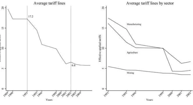
Figure 1
Tariff reductions in Indonesia
Cooperation (Fane 1999). Although the removal of specific nontariff barriers was accompanied by a temporary rise in tariffs (especially in the food manufacturing sector), this did not affect the overall declining trend in any major way.
Figure 1 shows the reduction in tariff lines over time and the variation between industries. On average, nominal tariffs reduced from 17.2 percent in 1993 to 6.6 percent in 2002. In this period the strongest reductions occurred from 1993 to 1995 and during the post crisis period after 1999. While tariffs decreased across the board, there were marked differences in initial levels and in the extent of the decrease. Manufacturing started with relatively high tariff barriers but also showed the stron-gest reductions. For example, wood and furniture saw tariffs decline from 27.2 to 7.9 percent, textiles from 24.9 to 8.1 percent, and other manufacturing from 18.9 to 6.4 percent. The average tariffs for agriculture were already much lower, reducing from 11.5 to 3.0 percent.
relative wages in the textile and apparel sector. Additionally, working conditions, proxied by workers’ own assessment of their income, working facilities, medical benefits, safety considerations, and transport opportunities, improved over time in the expanding manufacturing industries as compared to agriculture.
Based on a microsimulation exercise Hertel, Ivanic, Preckel, and Cranfield (2004) argue that full multilateral trade liberalization is expected to decrease household poverty in Indonesia, although self-employed agricultural households would be the most likely losers of trade liberalization in the short run, which is mainly due to the assumption that self-employed labor is immobile in the short run. In the longer run some former agricultural workers will be moving into the formal wage labor market and the poverty headcount could be expected to fall for all sectors. However, the mobility of low-skill labor, and hence the speed and ability to exploit the opportu-nities from trade liberalization, may be underestimated by Hertel et al. (2004). For example, Suryahadi, Suryadarma, and Sumarto (2009) show that during the 1990s the agriculture employment share dropped from 50 to 40 percent, while the services share increased from 33 to 42 percent. In addition, they attribute most of the poverty reductions in that decade to growth in urban services. This is further supported by Suryahadi (2001), who documents a fast increase in the employment of skilled labor force as well as a decline in wage inequality (faster wage growth for the unskilled) during trade liberalization in Indonesia, although he does not establish causality.
B. Child Work
Indonesia experienced a steady decline in child work in the 30 years before the Indonesian economic crisis, but this decline halted with the onset of the crisis (Sur-yahadi, Priyambada, and Sumarto 2005). Nevertheless, market work among children aged 10–15 increased only slightly in response to the economic crisis (Cameron 2001). During the crisis children have been moving out of the formal wage em-ployment sector into other small-scaled activities (Manning 2000), but the labor supply response seems to be concentrated with older cohorts.
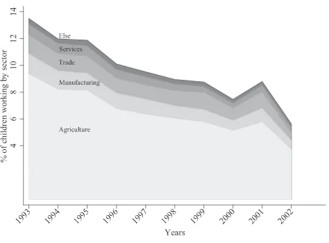
The overall decline in child work is portrayed in Figure 2, for boys and girls, and by different age groups. Child work is here defined as any work activity that con-tributes to household income. From 1993 to 2002, the incidence of child work halves for children of junior secondary school age (13–15 years old), and is cut by more than 70 percent for children age 10–12. This decline is observed for both boys and girls, although boys engage in market work more than girls. In 2002 market work incidence for boys age 13–15 years is 14.8 percent, and 2.3 percent at age 10–12. Among girls market work incidence is 10.0 and 1.6 percent for the same age groups, respectively.
’ ’
Figure 2
Work of children, by gender and age group
Figure 3
Sectoral distribution of child work (aged 10–15 years)
remains a problem. Other problems that are still cause for concern are delayed enrollment, relatively high repetition rates, teacher quality and absenteeism, and lack of access to secondary schools in remote and rural areas (World Bank 2006).
In the remainder of this analysis we focus on child work activities by primary school age children close to the transition point, age 10–12, and junior secondary school age children, age 13 to 15. For children younger than 10 information on work is not available.
IV. Data and Empirical Approach
A. DataIndonesia’s national socioeconomic household survey,Susenas, provides information on the outcome variables and socioeconomic characteristics for individuals and households. TheSusenasis conducted annually around January-February, typically sampling approximately 200,000 households, and is representative at the district level. The district will be our main unit of analysis, as districts take a key role as the main administrative units in Indonesia, and the regional labor markets also are best defined in district terms.
Districts are defined as municipalities (Kota) or predominantly rural areas (Ka-bupaten). Each district (both the Kota and Kabupaten) can be further divided into urban precincts (Kelurahan) and rural villages (Desa). It is important to emphasize the difference between these two urban/rural indicators, since we will use both vari-ables in our analysis. A district classified as a rural Kabupaten mainly consists of rural villages, but also may include small towns that are registered as urban precincts in the data. In a similar vein, districts classified as urban Kota mainly contain urban precincts and neighborhoods, but also may cover some rural areas at the fringes, which are then registered as villages.9The Kota/Kabupaten classification will there-fore appear as a fixed effect in our analysis, but we also will investigate the differ-ential effects of tariff reduction for municipalities and rural districts. In addition, we will include the Desa/Kelurahan division as time variant control variable within districts.
The outcome variables record whether a child has worked in the last week. As mentioned earlier, market work is defined as activities that directly generate house-hold income, irrespectively of whether it was performed at the formal labor market or within the family. We distinguish it from domestic work, which consists of house-hold chores only. The Susenas also provides information on education attainment of other household members, household composition, monthly household expenditure, and sector of employment.10
Information on tariff lines comes from the UNCTAD-TRAINS database. These reflect the simple average of all applied tariff rates, which tend to be substantially
lower than the bound tarrifs during the 1990s (WTO 1998; WTO 2003). As data on tariff lines is not available for some years (1994, 1997, and 1998), we use infor-mation from four three-year intervals (1993, 1996, 1999, and 2002) both in the pooled cross-section and in the district panel. We can consistently match the relevant product categories to sectoral employment data derived from Susenas at the one-digit level.
The sectoral share of GDP per district that we use for constructing an alternative tariff weighting scheme is derived from the Regional GDP (GRDP) data of the Central Bureau of Statistics in Indonesia (BPS). The district GRDP are available from 1993 onward, and breaks down district GDP by one-digit sector, of which the tradable sectors are agriculture, manufacturing, and mining/quarrying.
Some districts have been dropped from the analysis. Districts in Aceh, Maluku, and Irian Jaya have not been included in the Susenas in some years due to violent conflict situations at the time of the survey. In addition, the 13 districts in East Timor were no longer covered by Susenas after the 1999 referendum on independence. Another problem is that over the period 1993 to 2002 some districts have split up over time. To keep time consistency in the district definitions, we redefine the dis-tricts to the 1993 parent district definitions.
Since the Susenas rounds are representative for the district population in each year, we construct a district panel by pooling the four annually repeated cross-sections. This yields a balanced panel of 261 districts, which reduces to 244 districts when we use the GRDP data. In addition to the pooled data, we also create a district pseudo-panel by computing district-level means for each variable, weighted by sur-vey weights. The advantage of pooling the cross-section data is that we can work with individual level data and can account for individual heterogeneity. For example, we are interested in the differential impact for high- and low-skill labor, urban and rural areas, by birth order, and gender. On the other hand, in the pseudo-panel the observation unit is the district which allows us to investigate dynamic effects at the district level.11
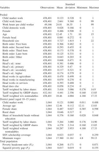
Table 1 provides descriptive statistics. Pooling the four years of Susenas data yields a sample of 458,401 observations for children age 10–15. The top panel of the table shows the outcome variables and the individual and household character-istics that we will use in the regressions. The bottom panel shows the descriptive statistics for the different tariff measures after they have been merged to the indi-vidual data. The table also reports the district specific poverty head count ratio (P0) and poverty severity (P2). The poverty measures are based on per capita expenditure data from Susenas and province-urban/rural specific poverty lines.12
B. Regional Tariff Exposure
Following Topalova (2005) and Edmonds et al. (2010), tariff exposure measures are constructed by combining information on geographic variation in sector composition
11. In order to allow for heterogeneity in the district panel, we construct it not only for the whole sample but also for subsamples, divided by age, gender, the household head’s education, birth order, and for rural and urban districts.
Table 1
Child market work 458,401 0.123 0.328 0 1
Child work hours 458,401 2.661 9.360 0 99
Work hours per child worker 49,166 24.81 16.35 1 99
Child domestic work 458,401 0.028 0.166 0 1
Female 458,401 0.486 0.500 0 1
Age 458,401 12.45 1.71 10 15
Female head 458,401 0.081 0.272 0 1
Household size 458,401 5.727 1.815 1 22
Birth order: First born 458,401 0.366 0.482 0 1
Birth order: Second born 458,401 0.293 0.455 0 1
Birth order: Third born 458,401 0.173 0.378 0 1
Birth order: Later born 458,401 0.125 0.331 0 1
Birth order: Other 458,401 0.043 0.203 0 1
Rural 458,401 0.668 0.471 0 1
Head’s ed.: none 458,401 0.381 0.486 0 1
Head’s ed.: primary 458,401 0.329 0.47 0 1
Head’s ed.: secondary 458,401 0.117 0.321 0 1
Head’s ed.: higher 458,401 0.174 0.379 0 1
Head works in agriculture 458,401 0.470 0.499 0 1
Head works in manufacturing 458,401 0.079 0.270 0 1
Head works in services 458,401 0.393 0.488 0 1
Head does else 458,401 0.058 0.234 0 1
Tariff weighted by labor shares 458,401 5.416 3.086 0.176 14.9
Tariff weighted by GRDP shares 432,161 4.441 2.356 0.160 13.85
Tariff weighted w/o nontradables 458,401 10.46 4.004 4.188 17.33
District panel (aged 10–15 years)
Child market work 1,044 0.121 0.080 0.011 0.488
Average age 1,044 12.46 0.112 12.11 13.03
Female share 1,044 0.487 0.027 0.385 0.598
Rural share 1,044 0.646 0.317 0 1
Share of household heads without education
1,044 0.376 0.160 0.028 0.848
Tariff weighted by labor shares 1,044 5.264 3.080 0.176 14.90
Tariff weighted by GRDP shares 976 4.278 2.314 0.160 13.85
Tariff weighted without nontradables
1,044 10.287 3.953 4.188 17.33
SSN scholarship coverage 1,044 0.023 0.037 0 0.259
Minimum wages 1,044 17.360 11.161 4.8 59.13
Total population
Poverty headcount ratio (P0) 1,044 0.268 0.171 0 0.871
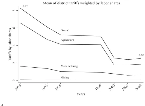
Figure 4
Evolution of tariff protection
of the economy and temporal variation in tariff lines by product category. This yields a measure indicating how changes in exposure to tariff reductions vary by geographic area over the period 1993 to 2002.
For each sector (h) the annual national tariff lines Tht for the relevant product
categories are weighted by the 1993 sector shares of active labor force (L) in district (k):
H
Lhk,1993 L
T ⳱ ⳯T
(1) kt
兺
冢
ht冣
L
h⳱1 k,1993
The evolution of tariff protection, weighted by employment shares, is shown in Figure 4.13This measure reflects how households are exposed to trade liberalization through local labor market dynamics. However, alternative measures of regional exposure to tariff reductions can be constructed, and we will probe into the robust-ness of our findings to the choice of tariff measure.
First, regional difference in economic sector composition, and hence relative ex-posure to tariff reductions, also could be expressed in terms of total output, instead of employment shares. Thus, we can define exposure by weighting tariff lines by the sectoral shares in GRDP:
H
This exposure measure differs considerably from exposure based on labor shares, as agriculture typically has relatively high employment but low economic production shares, while the opposite holds for manufacturing. This weighting scheme results in overall lower exposure since GRDP weights give a lower weight to agriculture than its importance in terms of employment.
Second, we explore the sensitivity of our results to excluding nontradables in the weighting scheme. By assigning nontraded goods and services a zero tariff, as in Topalova (2005) and Edmonds et al. (2010), our measure of tariff exposure will be relatively small in regions where the share of the nontradable (and hence not directly affected) sectors is large. However, Hasan, Mitra, and Ural (2007) criticize this approach, finding very different results to Topalova (2005) when they weight tariff changes across traded sectors only.14We therefore construct a similar measure of tariff exposure, based on labor shares of the tradable sectors only. Sensitivity to excluding not-tradables would imply that our results hinge on the size of the non-tradable sector in the regional economy.
Because regionally representative data on the sectoral composition of households is usually available only at the one- or two-digit level, we cannot distinguish tariff reductions on locally produced import-competing goods from tariff reductions on goods which are not produced locally. Instead, our focus lies on the interactions between overall trade liberalization and the regional differences in economic struc-ture, which determine the extent to which a region might be negatively affected by reductions in protection but also the extent to which it might be able to benefit from the efficiency gains associated with more competition in the local economy.
C. Identification
1. Static Analysis: Pooled District Panel
Identification of the impact of tariff reductions relies on the geographic panel nature of the combined data, and in particular on the variation in tariff exposure over districts and over time. We include district fixed effects (␦k), while time-region fixed
effects control for aggregate time trends (rt), allowing these to differ by the five
main geographic areas of the archipelago: the islands of Java, Sumatra, Kalimantan, and Sulawesi, and a cluster of smaller islands consisting of Bali and the Nusa Teng-gara group. We also include a set of time variant household and individual control variables (Xikt): a child’s age, gender, and birth order, the education, gender, and
main industry of occupation of the household head, the household size, and whether a household resides in an urban precinct or rural village (theDesa/Kelurahan com-position of districts).
The main specification for the pooled district panel is
⬘
Pr(y ⳱1)⳱Pr(␣ⳭT ⳭX ␥Ⳮ Ⳮ␦Ⳮε ⬎0)
(3) ikt kt ikt rt k ikt
whereyiktreflects work activities for childiin districtk at timet. We estimate the
model for the whole sample as well as separately for boys, girls, municipalities, and rural districts. The differential impact of trade liberalization is further explored by interacting tariff exposure with a set of individual chracteristics: the education as well as main occupation of the head of household (which also proxy for high- or low-skill labor) and the birth order of the children
2. Potential Sources of Bias
The main identifying assumption is that time variant shocks εikt are orthogonal to
Tkt. This would seem a reasonable assumption, given thatTktconsists of the baseline
economic structure and national changes in tariff regime. Thus, any temporal or regional variation endogenous to child work activities would be controlled for by time and geographic fixed effects. However, the identifying assumption would be violated if changes in district tariff exposure are endogenous to different local growth trajectories. Within the Indonesian context, regional variation in growth trajectories may be partly determined by initial conditions regarding sectoral composition.
A first trend to note is that districts with a higher initial incidence of child labor experience larger decreases in child labor over time. This occurs in particular in rural areas, with the bulk of child work located in agriculture. Regional diversity in structural change from the primary to secondary and tertiary sectors and in economic outcomes is a prominent feature of Indonesia’s economic geography. Hill, Resosu-darmo, and Vidyattama (2008) show evidence of strong regional variation in eco-nomic growth and structural change since the 1970s. However, they find only weak positive correlation between economic growth and structural change in districts. A related initial conditions problem, discussed at length by Edmonds et al. (2010), lies with the nontradable sector. Districts may experience different growth paths, de-pending on the size of the nontradable sector.
Because the initial sectoral composition of district economies is at the heart of Tkt, such differential trends in child labor could confound our estimates. We explore
the scope of these confounding effects through an initial conditions sensitivity anal-ysis and exploiting the panel features of the data.
Finally, social policy also could introduce confounding trends. Two policies are of particular concern for our analysis: changes in minimum wages and the 1998 crisis response. Minimum wages were introduced in Indonesia in the 1970s, and have increased strongly during the 1990s and between 2000 and 2002 (Alatas and Cameron 2008; Suryahadi et al. 2003). Minimum wage levels and changes vary by region and are influenced by local authorities. In 1998, in the wake of the economic crisis, a Social Safety Net (SSN) scholarship program was introduced to protect access to education for the poor. Sparrow (2007) finds that the scholarships decreased child labor, in particular for the poor and in rural areas. If regional variation in minimum wage levels or the impact of the scholarships is correlated with our tariff measure, then we may overestimate effects from trade liberalization on child labor. We therefore include minimum wage levels for provinces and the share of house-holds in districts that receive SSN scholarships (in 1999 and 2002) as time variant control variables.15
3. Dynamic Analysis: District Pseudo-Panel
Collapsing the pooled district panel to a district pseudo-panel provides more options to further address the potential source of bias and allows a dynamic analysis, at the cost of losing the individual variation in the data. The district pseudo-panel analogue to Equation 3 is
⬘ ¯
y¯ ⳱␣ⳭT ⳭX ␥Ⳮ Ⳮ␦Ⳮε¯
(4) kt kt ikt rt k kt
wherey¯ktis the fraction of children in districtkthat work in a given yeart.
This specification is still prone to bias through time variant unobservables. How-ever, with the fixed effects removed after a first-difference transformation of Equa-tion 4, it provides a first indicative test of exogeneity of tariff exposure. The as-sumption of strict exogeneity,E
{
Tkt ks¯ε}
⳱0for allsandt, implies thatTkt shouldadd no extra explanatory information in the regression
⬘ ¯
Dy¯ ⳱DT ⳭT ⳭDX ␥Ⳮ ⳭDε¯
(5) kt kt kt ikt rt kt
which provides the testable hypothesis that⳱0.
As suggested by Edmonds et al. (2010), the scope of the bias related to initial conditions can be investigated further by introducing initial sector shares as control variables. We therefore add initial conditions interacted with year dummy variables to Equation 5. Initial conditions are reflected by the 1993 labor shares of the agri-culture, mining, manufacturing, construction, trade, and transport sectors (with util-ities as reference group), in addition to adult literacy rates in districts. If our tariff measures are endogenous to child work, or if they capture differential trends in child work between districts, we also would expect child work to be correlated with future changes in district tariff exposure. We test this by regressing changes inyfrom 1993 to 1996 on changes inTfrom 1999 to 2002 (DTktⳭ2).
Finally, we exploit the pseudo-panel fully by taking a dynamic specification, where we include a lagged dependent variable and lagged tariff measure:
⬘ ¯
y¯ ⳱T ⳭT Ⳮy¯ ⳭX ␥Ⳮ Ⳮ␦Ⳮε¯
(6) kt kt ktⳮ1 ktⳮ1 ikt rt k kt
By including a lagged dependent variable we account for state dependence, and potential confounding differential trends in child labor between relatively high- and low-child labor districts. The lagged effects of tariff changes can identify short- and long-term effects. The immediate effect of a percentage point change in tariff ex-posure is reflected by. The total long-term change inyas a result of a percentage point change in tariff exposure, taking into account lagged effects of tariff changes and its dynamic multiplier effect troughy¯ , is approximated by (Ⳮ)/(1ⳮ).
ktⳮ1
suffi-cient identifying variation and to be good predictors of future changes. In particular, since our data observes a period of structural change, hence the changes do not follow a random walk. For instance, the reductions in tariffs are closely correlated with their initial levels (with reductions being the highest in high tariff sectors). For the instruments to be valid, lagged levels have to be orthogonal to the first diferenced error term. This seems a plausible assumption for tariffs, as the results of sensitivity analysis (see Section VB) suggest that strict exogeneity holds. For the lagged de-pendent the identifying assumption may be violated if there are higher order con-vergence effects, and ytⳮ2 affects Dyt other than through Dytⳮ1. We will test the validity of the instruments using a Hansen overidentifying restrictions test. System estimation, which would imply estimating a level equation along with the difference equation, is not suitable as this requires the identifying assumption that the instru-ments are not correlated with the fixed effects. This is a problematic assumption since a main cause of concern for our analysis lies with confounding fixed effects. This also is reflected in the Hansen test results, which strongly reject the validity of the instruments in case of system GMM.16
V. Results
A. Static AnalysisWe start by looking at the results from the static analysis, applying Specification 3 to pooled cross-section data. The estimated effects are given in Table 2. The table only reports the coefficients for tariff exposure, omitting the other covariates for ease of presentation.
The basic specification (Model A) indicates that a decrease in tariff exposure is associated with a decrease in child work for 10–15 year old children, but the size of the effect varies by gender and between urban and rural areas. A percentage point decrease in labor weighted tariff exposure leads to a 1.5 percentage point decrease in work incidence. The effect is somewhat stronger for boys than for girls with point estimates of 1.7 percentage points for boys and 1.2 for girls. These results are mainly driven by the effect in rural districts, where the estimates are larger and more precise than for municipalities (1.4 and 1.2 percentage points, respectively).
Model B investigates differential effects by skill level. The tariff exposure measure is interacted with the level of education of the head of household, defined as (i) not completed primary school, (ii) completed primary school, (iii) completed secondary school, and (iv) completed higher education. The benefits of tariff reductions are relatively higher for low-skill households; this is the first indicative evidence that poorer (lower-skilled) households might have benefited more from tariff reductions. The differential benefits for children from lower-skilled headed households are also larger for boys and in rural districts. These results are in line with general Stolper-Samuelson type expectations, and show that the favourable income effects to the
The
Journal
of
Human
Resources
Table 2
Pooled results: Child market work incidence (aged 10–15 years) and tariff protection
Sample All Male Female Rural Urban
(1) (2) (3) (4) (5)
Model A
Tariff 0.0145** 0.0166** 0.0123** 0.0145** 0.0115*
(0.0015) (0.0019) (0.0014) (0.0032) (0.0057)
AdjustedR2 0.137 0.164 0.118 0.138 0.120
Model B
Tariff⳯head’s education: none 0.0155** 0.0177** 0.0132** 0.0154** 0.0135*
(0.0015) (0.0019) (0.0015) (0.0032) (0.0063) Tariff⳯head’s education: primary 0.0129** 0.0150** 0.0107** 0.0134** 0.0127*
(0.0014) (0.0018) (0.0014) (0.0031) (0.0063) Tariff⳯head’s education: secondary 0.0093** 0.0103** 0.0082** 0.0103** 0.0071
(0.0014) (0.0018) (0.0015) (0.0030) (0.0052) Tariff⳯head’s education: higher 0.0049** 0.0059** 0.0039** 0.0054† 0.0090
(0.0014) (0.0018) (0.0015) (0.0030) (0.0062)
AdjustedR2 0.138 0.165 0.119 0.138 0.120
Model C
Tariff⳯head works in agriculture 0.0154** 0.0176** 0.0130** 0.0149** 0.0212*
(0.0015) (0.0019) (0.0014) (0.0031) (0.0101) Tariff⳯head works in manufacturing 0.0121** 0.0124** 0.0117** 0.0101** 0.0120*
(0.0020) (0.0025) (0.0019) (0.0035) (0.0057) Tariff⳯head works in services 0.0067** 0.0079** 0.0055** 0.0067* 0.0092
Kis-Katos
and
Sparrow
739
AdjustedR 0.138 0.165 0.119 0.138 0.120
Model D
Tariff⳯first born 0.0175** 0.0195** 0.0150** 0.0163** 0.0130*
(0.0016) (0.0019) (0.0015) (0.0032) (0.0056) Tariff⳯second born 0.0160** 0.0177** 0.0142** 0.0156** 0.0121*
(0.0015) (0.0020) (0.0015) (0.0032) (0.0059) Tariff⳯third born 0.0130** 0.0139** 0.0119** 0.0129** 0.0052
(0.0015) (0.0019) (0.0014) (0.0031) (0.0056) Tariff⳯later born 0.0097** 0.0105** 0.0087** 0.0092** 0.0104†
(0.0015) (0.0019) (0.0015) (0.0031) (0.0054) Tariff⳯other relatives 0.0041 0.0149** ⳮ0.0050 0.0124** 0.0406
(0.0030) (0.0026) (0.0042) (0.0033) (0.0274)
AdjustedR2 0.138 0.165 0.120 0.145 0.121
Number of observations 458,401 235,390 223,011 375,400 83,001
Number of districts 261 261 261 209 52
poor must have dominated eventual substitution effects arising from increasing un-skilled wages.
A similar picture arises when differentiating the tariff effects by sector of main occupation of the household head (Model C). We distinguish between the three main sectors (agriculture, mining/manufacturing, and services) and a fourth category that includes other unclassified occupations and those inactive. The effects of tariff re-ductions are strongest for children from agricultural and manufacturing (and hence once again poorer) households, with the effects being somewhat larger, but also less precise, in urban districts. We also see beneficial effects for children in households where the head works in a fully protected sector (like services) or is inactive. This might be due to the overall poverty reducing effects of trade liberalization in the region.
The size of the estimated effect of tarif exposure decreases with the birth order of a child (Model D). The regressions show the differential estimates for the first three children born to a household, latter borns, and other relatives (which includes children from servants). The effect is much stronger for the first- and second-born. This is consistent with other findings that labour supply of older children in house-holds is more responsive to postive shocks due to social policy reforms as compared to their younger siblings (Sparrow 2007). For other relatives and servants we do not find a decrease for girls, only for boys.
Our measure of child work incidence ignores changes in child work hours by children that remain active in the labor market, in which case we may not capture the full impact of trade reforms. We therefore also explore the effects on work hours for boys and girls. The point estimates for work incidence and hours are similar in order of magnitude when compared to initial sample averages. Moreover, that sub-sequent GMM analysis with the pseudo-panel yields very similar results for work incidence and work hours. This would suggest that the estimated effect on work incidence provides a fair representation of the impact on child labor. The remainder of the analysis will therefore focus on work incidence.17
B. Sensitivity Analysis and Exogeneity Tests
The static results are based on district fixed effects, and could be confounding the effects of trade liberalization and differential growth paths. This section will examine this potential source of bias. The pseudo-panel first-difference results are presented in Table 3. Column 1 shows that the effects of tariff changes on child work remain precise and are consistent with the pooled cross-section results, although the coef-ficients are slightly smaller, at 0.9 percentage point. There is no evidence of con-founding social policy effects, as the tariff coefficients are robust to including the minimum wage and SSN scholarship variables (Column 2).18 The test for strict
17. These results for work hours are reported in the supplemental appendix. As working children form a selective sample, we both present OLS and Tobit estimates on the weekly hours of work for all children. We also estimated the effects on domestic work (not shown here), which are small and not statistically significant, and therefore also ignored in the remainder of the analysis.
Kis-Katos
and
Sparrow
741
D Child market work
1993–2002 1993–1996 1999–2002 Dependent
Time period (1) (2) (3) (4) (5) (6) (7)
DTariffs 0.0094** 0.0093** 0.0078** 0.0099 0.0088** 0.0102** (0.0015) (0.0015) (0.0027) (0.0090) (0.0027) (0.0027)
Tariffs ⳮ0.0012 0.0049
(0.0016) (0.0043)
DTariffstⳭ2 ⳮ0.0027
(0.0017)
R2 0.201 0.202 0.202 0.341 0.130 0.136 0.317
Number of observations 783 783 783 783 522 261 261
Further controls Yes Yes Yes Yes Yes Yes Yes
Social policy variables No Yes Yes Yes No No No
Initial conditions⳯year
interactions
No No No Yes No No No
Number of districts 261 261 261 261 261 261 261
exogeneity of tariffs exposure with respect to child work in Column 3 does not reject the zero hypothesis of strict exogeneity. The estimated effect on child work also is robust to including the initial conditions of sector shares, the adult literacy rate, and child market work incindence, interacted with year dummy variables (Column 4), although the estimate loses precision when the interaction terms are included.19 Fi-nally, we find no correlation between child work and future tariff changes (Column 5). Summarizing, the results from Table 3 suggest that the negative relationship between tariff reduction and child work is not driven by omitted variables, or dif-ferential growth trajectories of district economies, and the reduction of the agricul-tural sector.
The economic crisis in 1997/98 also raises interpretational concerns, as the de-valuation of the Rupiah resulted in short-term price spikes that affected especially the poor. Although the effect of the price spike has largely subsided by the 1999 Susenas round, and the overall negative effect of the crisis is controlled for by the region-time fixed effects, concerns may still remain that the crisis confounds the effects of tariff reductions. This is especially the case if the effects of the crisis were correlated with the economic structure of the districts. In order to investigate these concerns, Columns 6 and 7 of Table 3 report difference estimates for two separated time periods: 1993–96 (precrisis) and 1999–2002 (postcrisis). The results confirm the robustness of our findings, as they are largely unaffected by the split.
C. Dynamic Analysis
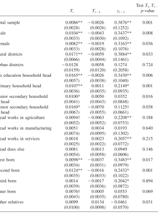
The main GMM estimation results for the dynamic specification are summarized in Table 4, by gender, for rural and urban districts, by household head’s education level and occupation category, and by birth order.20 The results suggest that the local effects of tariff reductions are considerable: decreasing district tariff exposure by one percentage point leads to a decrease in child labor incidence of the 10–15 years old by around 0.9 percentage points. Recursive substitution over the four periods gives us an indication of the overall effect of the decrease in local tariff exposure: the tariff reductions explain around 70 percent of the average reduction of child labor of 9.0 percentage points. We also see some evidence of convergence, with a coefficient for the lagged dependent of 0.39, suggesting (changes in) child labor to decrease over time.
19. It also could be that convergence drives our results, if child labor decreases faster in districts with initial high child labor, which in turn would be correlated with the district tariff measures. We investigate this possible source of bias by introducing a lagged level of child labor in a difference specification of the dynamic model described in Equation 6. The results do provide evidence of convergence, but we find that the estimates for tariff changes are robust and remain statistically significant. These results are reported in the supplemental appendix.
Table 4
Child market work incidence (aged 10–15 years) and tariff protection, difference GMM estimates
TestTt,Ttⳮ1
Tt Ttⳮ1 ytⳮ1 p-value
Total sample 0.0086** ⳮ0.0026 0.3876** 0.001 (0.0028) (0.0026) (0.1252)
Male 0.0104** ⳮ0.0043 0.3437** 0.008
(0.0033) (0.0030) (0.1092)
Female 0.0082** ⳮ0.0019 0.3163** 0.036
(0.0033) (0.0028) (0.1076)
Rural districts 0.0171** ⳮ0.0059 0.3884** 0.033 (0.0066) (0.0044) (0.1461)
Urban districts ⳮ0.0128 0.0058 0.1274 0.724
(0.0159) (0.0120) (0.2058)
No education household head 0.0165** ⳮ0.0026 0.3430** 0.006 (0.0057) (0.0038) (0.1040)
Primary household head 0.0107** 0.0011 0.2149* 0.001 (0.0036) (0.0035) (0.0935)
Head works in agriculture 0.0094† ⳮ0.0063 0.2208** 0.188
(0.0052) (0.0052) (0.0753)
Head works in manufacturing 0.0051 0.0034 0.0193 0.640 (0.0074) (0.0095) (0.1302)
Head works in services 0.0018 0.0023 0.2057** 0.215 (0.0025) (0.0022) (0.0772)
Head does else 0.0081 0.0013 0.0949 0.146
(0.0054) (0.0058) (0.0606)
First born 0.0098** ⳮ0.0037 0.3483** 0.017 (0.0034) (0.0031) (0.0979)
Second born 0.0124** ⳮ0.0016 0.2432* 0.001
(0.0035) (0.0033) (0.1022)
Third born 0.0014 ⳮ0.0017 0.2042* 0.894
(0.0039) (0.0036) (0.0872)
Later born 0.0076† 0.0005 0.0553 0.069
(0.0043) (0.0035) (0.0780)
Other relatives 0.0099 0.0134 ⳮ0.0461 0.031
(0.0100) (0.0098) (0.0570)
The gender gap favors boys slightly and is comparable in magnitude to the pooled estimates. Decomposing the tariff effects for the rural and urban subsamples, these favorable effects appear to be mainly rural as we do not find robust effects for the urban districts. Child labor outcomes improve irrespective of household skill com-position and these effects are only statistically significant in agricultural households and in the remainder category. The GMM results do not monotonically change by birth order, with the first and second born benefiting most from tariff reductions.
Our study remains largely a reduced form analysis, and we are not able to identify the main transmission channels through which child work is affected by reduced tariff exposure. Nevertheless, we can provide some global indication of the main mechanisms at work, by looking at the effects on district poverty profiles and adult employment.
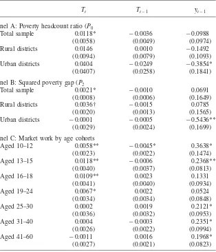
Tariff reductions have led to a reduction in the extent and severity of poverty. Table 5 shows the estimated effects of reduced tariff exposure on the poverty head count ratio (Panel A) and the squared poverty gap (Panel B), where the model specification is similar to the earlier dynamic GMM. While the poverty head count merely records the fraction of the district population that cross an arbitrary level of consumption, the squared poverty gap reflects the curvature in the per capita expen-diture distribution for the population living below the poverty line. The results show that a percentage point reduction in tariff exposure reduces the poverty headcount in districts by 1.2 percentage point, and also reduces inequality among the poor. In other words, the results seem to suggest that income effects play a role, in particular at the bottom end of the income distribution.
Addressing changes in workfoce participation by age category (Panel C), we see the strongest effects of tariff reductions for the age group of 13–15 years old, which is not surprising given the low incidence of child work among primary school age children. Moreover, tariff reductions do not impact workforce participation of co-horts older than 18. This would suggest that the effect of trade liberalization on child labor is not driven by substitution of child for adult labor, and that the observed income effects are not due to a labor supply response and reduced unemployment. Rather, income effects seem to be a result of relative wage increases, in particular for low-skill labor.
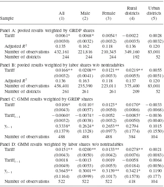
D. Alternative Measures of Tariff Exposure
Estimates for alternative measures of tariff exposure are given in Table 6. Compared to the results weighted by labor shares, the estimated effects are smaller and less precise for GRDP weighted tariff exposure in case of the pooled data (Panel A), but are very much consistent with the pseudo-panel GMM results (Panel C). The results are robust to the manner in which nontraded goods are incorporated in the tariff exposure measure. Panels B and D show the results when we focus on tradable sector composition only, for the pooled and GMM analysis, respectively. The main differences observed when excluding the size of the nontradable sector from the weighting scheme is that both the gender and urban/rural gaps increase considerably, as the benefits of tariff reductions seem skewed to boys and urban households.21
Table 5
Tariff reductions and potential channels, difference GMM estimates
Tt Ttⳮ1 ytⳮ1
Panel A: Poverty headcount ratio (P0
Total sample 0.0118* ⳮ0.0036 ⳮ0.0988
(0.0058) (0.0049) (0.0974)
Rural districts 0.0146 0.0010 ⳮ0.1492
(0.0094) (0.0079) (0.1093)
Urban districts 0.0404 ⳮ0.0249 ⳮ0.3854*
(0.0407) (0.0258) (0.1841)
Panel B: Squared poverty gap (P2
Total sample 0.0021* ⳮ0.0010 0.0691
(0.0008) (0.0006) (0.1649)
Rural districts 0.0036† ⳮ0.0015 0.0785
(0.0020) (0.0013) (0.1565)
Urban districts ⳮ0.0001 ⳮ0.0005 ⳮ0.5436**
(0.0029) (0.0024) (0.1699)
Panel C: Market work by age cohorts
Aged 10–12 0.0058** ⳮ0.0045* 0.3638*
(0.0023) (0.0022) (0.1474)
Aged 13–15 0.0118** ⳮ0.0006 0.2368**
(0.0040) (0.0037) (0.0813)
Aged 16–18 0.0109** 0.0023 0.1331
(0.0041) (0.0040) (0.0934)
Aged 19–24 0.0067* 0.0022 0.0524
(0.0034) (0.0034) (0.0848)
Aged 25–30 0.0002 0.0019 0.2121*
(0.0036) (0.0032) (0.0953)
Aged 31–40 0.0004 ⳮ0.0003 0.2351*
(0.0026) (0.0022) (0.0994)
Aged 41–60 ⳮ0.0011 0.0016 0.1968*
(0.0027) (0.0021) (0.0823)
Notes: Coefficients are presented in rows for different subsamples. Models in Panel A and B include region and time interactions, rural share, lagged per capita GRDP, and adult literacy. The lagged dependent tariffs, rural share, lagged per capita GRDP, and adult literacy are treated as endogenous. Models in Panel C have a similar specification as in Table 4. Robust standard errors are in parentheses.N⳱508 in the total, 416 in the rural, and 92 in the urban sample;N⳱522 in Panel C. **, *, † denote significance at the 1, 5, and 10 percent level.
VI. Conclusion
bar-Table 6
Robustness to alternative tariff protection measures
All Male Female
Rural districts
Urban districts
Sample (1) (2) (3) (4) (5)
Panel A: pooled results weighted by GRDP shares
Tariff 0.0061* 0.0068* 0.0054† ⳮ0.0022 0.0028 (0.0030) (0.0032) (0.0032) (0.0035) (0.0032)
AdjustedR2 0.135 0.162 0.118 0.136 0.120
Number of observations 432,161 221,816 210,345 349,160 83,001
Number of districts 244 244 244 192 52
Panel B: pooled results weighted by labor shares w/o nontradables
Tariff 0.0166** 0.0208** 0.0121** 0.0219** 0.0055 (0.0032) (0.0041) (0.0033) (0.0055) (0.0051)
AdjustedR2 0.136 0.163 0.118 0.137 0.120
Number of observations 458,401 235,390 223,011 375,400 83,001
Number of districts 261 261 261 209 52
Panel C: GMM results weighted by GRDP shares
Tariff 0.0106* 0.0110† 0.0123* 0.0170* ⳮ0.0033 (0.0043) (0.0057) (0.0050) (0.0086) (0.0068) Tarifftⳮ1 ⳮ0.0060† ⳮ0.0074† ⳮ0.0052 ⳮ0.0085† ⳮ0.0036
(0.0032) (0.0038) (0.0032) (0.0050) (0.0040)
ytⳮ1 0.3338* 0.2624* 0.2653** 0.2794 0.1015
(0.1379) (0.1328) (0.0977) (0.1774) (0.1550) Number of observations 488 488 488 384 104
Panel D: GMM results weighted by labor shares w/o nontradables
Tariff 0.0151** 0.0200** 0.0133** 0.0278** 0.0021 (0.0043) (0.0050) (0.0042) (0.0076) (0.0083) Tarifftⳮ1 0.0018 ⳮ0.0013 0.0019 ⳮ0.0058 0.0064
(0.0049) (0.0053) (0.0055) (0.0184) (0.0056)
ytⳮ1 0.3645** 0.3001** 0.3139** 0.3421* 0.1190
(0.1164) (0.0999) (0.1017) (0.1578) (0.177) Number of observations 522 522 522 418 104
Notes: For Panels A and B see the notes to Table 2, for Panels C and D see the notes to Table 5. **, *, † denote significance at the 1, 5, and 10 percent level.
riers, as average import tariff lines decreased from 17.2 percent in 1993 to 6.6 percent in 2002; a period that also saw reductions in child work.
effects of trade policy. The results are robust to specification and sensitivity analysis, and we find no evidence of remaing sources of bias.
Our main findings suggest that Indonesia’s trade liberalization experience in the 1990s has contributed to a strong decline in child labor, as decreased tariff exposure is associated with a decrease in work by 10–15-year-old children. The effects of tariff reductions increase with the age of children and decrease with their birth order, and are strongest for children from low-skill backgrounds and in rural areas. Through these effects, trade liberalization will have long-term welfare implications for human capital investments, in particular for low-skill, and presumably poorer, households. Although our reduced form analysis can at best provide indirect evidence of the main transmission channels, we do find strong support for the hypothesis that re-duction of child labor is driven by positive income effects from trade liberalization for the poorest. This is consistent with other studies, which argue that trade liber-alization in Indonesia brought about a relative wage increase for low-skill labor, although causal effects are hard to confirm (Suryahadi 2001; Arnold and Smarzynska Javorcik 2005; Sitalaksmi et al. 2007). Further analysis of this causal relationship would be an area of future research.
The findings in this paper and mixed empirical evidence from other country stud-ies would suggest that the potential benefits to be gained from trade liberalization, and its distributional implications, are indeed context-specific. The Indonesian con-text seems to have provided the preconditions needed to generate classic Stolper-Samuelson effects, partly facilitated by a coinciding process of structural change in the 1990s that saw a reallocation of labor from agriculture to services and manu-facturing. In particular the mobility of low-skill labor seems to play an important role, which, combined with increased productivity and competitiveness, has led to better employment opportunities outside agriculture and increased returns to low-skill labor. Such cross-country heterogeneinty may be underlying the weak average effects of trade liberalization on child labor and human capital investments found at macro level, highlighting the importance of considering local economic contexts when propagating trade reforms and formulating subsequent social policy responses.
References
Alatas, Vivi, and Lisa A. Cameron. 2008. “The Impact of Minimum Wages on Employment in a Low-Income Country: A Quasi-Natural Experiment in Indonesia.”Industrial and Labor Relations Review61(2):201–23.
Amiti, Mary, and Joep Konings. 2007. “Trade Liberalization, Intermediate Inputs and Productivity: Evidence from Indonesia.”American Economic Review97(5):1611–38. Arellano, Manuel, and Stephen Bond. 1991. “Some Tests of Specification for Panel Data:
Monte Carlo Evidence and an Application to Employment Equations.”Review of Economic Studies58(2):277–97.
Basri, M. Chatib, and Hal Hill. 2004. “Ideas, Interests and Oil Prices: The Political Economy of Trade Reform During Soeharto’s Indonesia.”The World Economy27(5):633– 55.
Beegle, Kathleen, Rajeev H. Dehejia, and Roberta Gatti. 2006. “Child Labor and Agricultural Shocks.”Journal of Development Economics81(1):80–96.
Bhagwati, Jagdish, and T. N. Srinivasan. 2002. “Trade and Poverty in the Poor Countries.”
American Economic Review92(2):180–83.
Cameron, Lisa A. 2001. “The Impact of the Indonesian Financial Crisis on Children: An Analysis using the 100 Villages Survey.”Bulletin of Indonesian Economic Studies
37(1):43–64.
Chiquiar, Daniel. 2008. “Globalization, Regional Wage Differentials and the Stolper-Samuelson Theorem: Evidence from Mexico.”Journal of International Economics
74(1):70–93.
Cigno, Alessandro, Furio Camillo Rosati, and Lorenzo Guarcello. 2002. “Does Globalisation Increase Child Labour?”World Development30(9):1579–89.
Davis, Donald R., and Prachi Mishra. 2007. “Stolper-Samuelson is Dead: And Other Crimes of Both Theory and Data.” InGlobalization and Poverty, NBER Chapters, ed. A. Harrison, 87–108. Chicago: University of Chicago Press for NBER.
Edmonds, Eric V., and Nina Pavcnik. 2005a. “Child Labor in a Global Economy.”Journal of Economic Perspectives8(1):199–220.
Edmonds, Eric V., and Nina Pavcnik. 2005b. “The Effect of Trade Liberalization on Child Labor.”Journal of International Economics65(2):401–19.
Edmonds, Eric V., and Nina Pavcnik. 2006. “International Trade and Child Labor: Cross– Country Evidence.”Journal of International Economics68(1):115–40.
Edmonds, Eric V., Nina Pavcnik, and Petia Topalova. 2010. “Trade Adjustment and Human Capital Investments: Evidence from Indian Tariff Reform.”American Economic Journal: Applied Economics2(4):42–75.
Fane, George. 1999. “Indonesian Economic Policies and Performance, 1960–98.”World Economy22(5):651–68.
Harrison, Ann. 2007.Globalization and Poverty.NBER Books. Chicago: University of Chicago Press for NBER.
Hasan, Rana, Devashish Mitra, and Beyza P. Ural. 2007. “Trade Liberalization, Labor-Market Institutions and Poverty Reduction: Evidence from Indian States.”India Policy Forum3:71–122.
Hertel, Thomas W., Maros Ivanic, Paul V. Preckel, and John A. L. Cranfield. 2004. “The Earnings Effects of Multilateral Trade Liberalization: Implications for Poverty.”The World Bank Economic Review18(2):205–36.
Hill, Hal, Budy P. Resosudarmo, and Yogi Vidyattama. 2008. “Indonesia’s Changing Economic Geography.”Bulletin of Indonesian Economic Studies44(3):407–35. Jafarey, Saqib, and Sajal Lahiri. 2002. “Will Trade Sanctions Reduce Child Labour?”
Journal of Development Economics68(1):137–56.
Jones, Gawin W., and Peter Hagul. 2001. “Schooling in Indonesia: Crisis-Related and Longer-Term Issues.”Bulletin of Indonesian Economic Studies37(2):207–31. Kis-Katos, Krisztina. 2007. “Does Globalization Reduce Child Labor?”Journal of
International Trade and Economic Development16(1):71–92.
Kis-Katos, Krisztina and Gu¨nther G. Schulze. Forthcoming. “Child Labor in Indonesian Small Industries.”Journal of Development Studies.
Kis-Katos, Krisztina and Robert Sparrow. 2009. “Child Labor and Trade Liberalization in Indonesia.” IZA Discussion Paper #4376. Bonn: Institute for the Study of Labor. Komiya, Ryutaro. 1967. “Non-Traded Goods and the Pure Theory of International Trade.
Manning, Chris. 2000. “The Economic Crisis and Child Labor in Indonesia.” ILO/IPEC Working Paper. Geneva: International Labour Office.
Ranjan, Priya. 2001. “Credit Constraints and the Phenomenon of Child Labor.”Journal of Development Economics64(1):81–102.
Sitalaksmi, Sari, Poppy Ismalina, Ardyanto Fitrady, and Raymond Robertson. 2007. “Globalization and Working Conditions: Evidence from Indonesia.” InGlobalization, Wages, and the Quality of Jobs: Five Country Studies, ed. R. Robertson, D. Brown, G. Pierre, and L. Sanchez-Puerta, 203–36. Washington D.C.: World Bank Publications. Sparrow, Robert. 2007. “Protecting Education for the Poor in Times of Crisis: An
Evaluation of a Scholarship Programme in Indonesia.”Oxford Bulletin of Economics and Statistics69(1):99–122.
Suryahadi, Asep. 2001. “International Economic Integration and Labor Markets: The Case of Indonesia.” Economics Study Area Working Paper #22, Honolulu: East-West Center. Suryahadi, Asep, Wenefrida Widyanti, Daniel Perwira, and Sudarno Sumarto. 2003.
“Minimum Wage Policy and its Impact on Employment in the Urban Formal Sector.”
Bulletin of Indonesian Economic Studies39(1):29–50.
Suryahadi, Asep, Agus Priyambada, and Sudarno Sumarto. 2005. “Poverty, School and Work: Children During the Economic Crisis in Indonesia.”Development and Change
36(2):351–73.
Suryahadi, Asep, Sudarno Sumarto, and Lant Pritchett. 2003. “Evolution of Poverty During the Crisis in Indonesia.”Asian Economic Journal17(3):221–41.
Suryahadi, Asep, Daniel Suryadarma, and Sudarno Sumarto. 2009. “The Effects of Location and Sectoral Components of Economic Growth on Poverty: Evidence from Indonesia.”
Journal of Development Economics89(1):109–17.
Topalova, Petia. 2005. “Trade Liberalization, Poverty, and Inequality: Evidence from Indian Districts.” NBER Working Paper #11614. Cambridge, Mass.: National Bureau of Economic Research.
Verhoogen, Eric. 2008. “Trade, Quality Upgrading, and Wage Inequality in the Mexican Manufacturing Sector.”Quarterly Journal of Economics123(2):489–530.
Windmeijer, Frank. 2005. “A Finite Sample Correction for the Variance of Linear Efficient Two-Step GMM Estimators.”Journal of Econometrics126(1):25–51.