Dynamic Trading with Predictable Returns
and Transaction Costs
NICOLAE G ˆARLEANU and LASSE HEJE PEDERSEN∗
ABSTRACT
We derive a closed-form optimal dynamic portfolio policy when trading is costly and security returns are predictable by signals with different mean-reversion speeds. The optimal strategy is characterized by two principles: (1) aim in front of the target, and (2) trade partially toward the current aim. Specifically, the optimal updated portfolio is a linear combination of the existing portfolio and an “aim portfolio,” which is a weighted average of the current Markowitz portfolio (the moving target) and the expected Markowitz portfolios on all future dates (where the target is moving). Intuitively, predictors with slower mean-reversion (alpha decay) get more weight in the aim portfolio. We implement the optimal strategy for commodity futures and find superior net returns relative to more naive benchmarks.
ACTIVE INVESTORS AND ASSET managers—such as hedge funds, mutual funds,
and proprietary traders—try to predict security returns and trade to profit from their predictions. Such dynamic trading often entails significant turnover and transaction costs. Hence, any active investor must constantly weigh the expected benefit of trading against its costs and risks. An investor often uses different return predictors, for example, value and momentum predictors, and these have different prediction strengths and mean-reversion speeds—put dif-ferently, different “alphas” and “alpha decays.” The alpha decay is important because it determines how long the investor can enjoy high expected returns, and therefore affects the trade-off between returns and transaction costs. For instance, while a momentum signal may predict that the IBM stock return will be high over the next month, a value signal might predict that Cisco will perform well over the next year.
∗G ˆarleanu is at Haas School of Business, University of California, Berkeley, NBER, and CEPR, and Pedersen is at New York University, Copenhagen Business School, AQR Capital Management, NBER, and CEPR. We are grateful for helpful comments from Kerry Back; Pierre Collin-Dufresne; Darrell Duffie; Andrea Frazzini; Esben Hedegaard; Ari Levine; Hong Liu (discussant); Anthony Lynch; Ananth Madhavan (discussant); Mikkel Heje Pedersen; Andrei Shleifer; and Humbert Suarez; as well as from seminar participants at Stanford Graduate School of Business, AQR Capital Management, University of California at Berkeley, Columbia University, NASDAQ OMX Economic Advisory Board Seminar, University of Tokyo, New York University, University of Copenhagen, Rice University, University of Michigan Ross School, Yale University School of Management, the Bank of Canada, and the Journal of Investment Management Conference. Pedersen gratefully acknowledges support from the European Research Council (ERC grant no. 312417) and the FRIC Center for Financial Frictions (grant no. DURF102).
DOI: 10.1111/jofi.12080
This paper addresses how the optimal trading strategy depends on securities’ current expected returns, the evolution of expected returns in the future, se-curities’ risks and return correlations, and their transaction costs. We present a closed-form solution for the optimal dynamic portfolio strategy, giving rise to two principles: (1) aim in front of the target, and (2) trade partially toward the current aim.
To see the intuition for these portfolio principles, note that the investor would like to keep his portfolio close to the optimal portfolio in the absence of transaction costs, which we call the “Markowitz portfolio.” The Markowitz
portfolio is a moving target, since the return-predicting factors change over
time. Due to transaction costs, it is obviously not optimal to trade all the way to the target all the time. Hence, transaction costs make it optimal to slow down trading and, interestingly, to modify the aim, and thus not to trade
directly toward thecurrentMarkowitz portfolio. Indeed, the optimal strategy
is to trade toward an “aim portfolio,” which is a weighted average of the current Markowitz portfolio (the moving target) and the expected Markowitz portfolios on all future dates (where the target is moving).
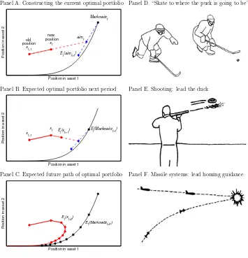
Panel A of Figure1illustrates the construction of the optimal portfolio of two
securities.1The solid line illustrates the expected path of the Markowitz
portfo-lio, starting with large positions in both security 1 and security 2, and gradually converging toward its long-term mean (for example, the market portfolio). The aim portfolio is a weighted average of the current and future Markowitz port-folios so it lies in the “convex hull” of the solid line. The optimal new position is achieved by trading partially toward this aim portfolio. Another way to state our portfolio principle is that the best new portfolio is a combination of (1) the current portfolio (to reduce turnover), (2) the Markowitz portfolio (to partly get the best current risk-return trade-off), and (3) the expected optimal portfolio in the future (a dynamic effect).
While new to finance, these portfolio principles have close analogues in other fields such as the guidance of missiles toward moving targets, hunting, and sports. The most famous example from the sports world is perhaps the following
quote, illustrated in Panel D of Figure1:
“A great hockey player skates to where the puck is going to be, not where it
is.” — Wayne Gretzky
Similarly, hunters are reminded to “lead the duck” when aiming their
weapon, as seen in Panel E.2
Panel B of Figure1illustrates the expected trade at the next trading date,
and Panel C shows how the optimal position is expected to chase the Markowitz portfolio over time. The expected path of the optimal portfolio resembles that of
1Panels A–C of the figure are based on simulations of our model. We are grateful to Mikkel
Heje Pedersen for Panels D–F. Panel F is based on “Introduction to Rocket and Guided Missile Fire Control,” Historic Naval Ships Association (2007).
Panel A. Constructing the current optimal portfolio
x t−1
x t
old position
new position
Markowitzt
aim t
E t(aimt+1)
Position in asset 1
Position in asset 2
Panel B. Expected optimal portfolio next period
Position in asset 1
Position in asset 2
x t−1
x
t Et(xt+1) Et(Markowitzt+1)
Panel C. Expected future path of optimal portfolio
E
t(Markowitzt+h) E
t(xt+h)
Position in asset 1
Position in asset 2
Panel D. “Skate to where the puck is going to be”
Panel E. Shooting: lead the duck
Panel F. Missile systems: lead homing guidance
Figure 1. Aim in front of the target.Panels A–C show the optimal portfolio choice with two securities. The Markowitz portfolio is the current optimal portfolio in the absence of transaction costs: the target for an investor. It is a moving target, and the solid curve shows how it is expected to mean-revert over time (toward the origin, which could be the market portfolio). Panel A shows how the optimal time-t trade moves the portfolio from the existing value xt−1toward the aim
portfolio, but only part of the way. Panel B shows the expected optimal trade at timet+1. Panel C shows the entire future path of the expected optimal portfolio. The optimal portfolio “aims in front of the target” in the sense that, rather than trading toward the current Markowitz portfolio, it trades toward the aim, which incorporates where the Markowitz portfolio is moving. Our portfolio principle has analogues in sports, hunting, and missile guidance as seen in Panels D–F.
a guided missile chasing an enemy airplane in so-called “lead homing” systems, as seen in Panel F.
The optimal portfolio is forward-looking and depends critically on each return
predictor’s mean-reversion speed (alpha decay). To see this in Figure1, note the
position in security 1 decays more slowly than that in security 2, as the predictor that currently “likes” security 1 is more persistent. Therefore, the aim portfolio loads more heavily on security 1, and consequently the optimal trade buys more shares in security 1 than it would otherwise.
We show that it is in fact a general principle that predictors with slower mean-reversion (alpha decay) get more weight in the aim portfolio. An investor facing transaction costs should trade more aggressively on persistent signals than on fast mean-reverting signals: the benefits from the former accrue over longer periods, and are therefore larger.
The key role played by each return predictor’s mean-reversion is an impor-tant new implication of our model. It arises because transaction costs imply that the investor cannot easily change his portfolio and therefore must consider his optimal portfolio both now and in the future. In contrast, absent transaction costs, the investor can reoptimize at no cost and needs to consider only current investment opportunities without regard to alpha decay.
Our specification of transaction costs is sufficiently rich to allow for both purely transitory and persistent costs. With persistent transaction costs, the price changes due to the trader’s market impact persist for a while. Since we fo-cus on market-impact costs, it may be more realistic to consider such persistent effects, especially over short time periods. We show that, with persistent trans-action costs, the optimal strategy remains to trade partially toward an aim portfolio and to aim in front of the target, though the precise trading strategy is different and more involved.
Finally, we illustrate our results empirically in the context of commodity futures markets. We use returns over the past 5 days, 12 months, and 5 years to predict returns. The 5-day signal is quickly mean-reverting (fast alpha decay), the 12-month signal mean-reverts more slowly, whereas the 5-year signal is the most persistent. We calculate the optimal dynamic trading strategy taking transaction costs into account and compare its performance to both the optimal portfolio ignoring transaction costs and a class of strategies that perform static (one-period) transaction cost optimization. Our optimal portfolio performs the best net of transaction costs among all the strategies that we consider. Its net Sharpe ratio is about 20% better than that of the best strategy among all the static strategies. Our strategy’s superior performance is achieved by trading at an optimal speed and by trading toward an aim portfolio that is optimally tilted toward the more persistent return predictors.
We also study the impulse-response of the security positions following a shock to return predictors. While the no-transaction-cost position immediately jumps up and mean-reverts with the speed of the alpha decay, the optimal position increases more slowly to minimize trading costs and, depending on the alpha decay speed, may eventually become larger than the no-transaction-cost position, as the optimal position is reduced more slowly.
The paper is organized as follows. Section Idescribes how our paper
con-tributes to the portfolio selection literature that starts with Markowitz (1952).
closed-form solution illustrates several intuitive portfolio principles that are
difficult to see in the models following Constantinides (1986), where the
solu-tion requires complex numerical techniques even with asinglesecurity andno
return predictors (i.i.d. returns). Indeed, we uncover the role of alpha decay and the intuitive aim-in-front-of-the-target and trade-toward-the-aim princi-ples, and our empirical analysis suggests that these principles are useful.
SectionIIlays out the model with temporary transaction costs and the
solu-tion method. Secsolu-tionIIIshows the optimality of aiming in front of the target
and trading partially toward the aim. SectionIVsolves the model with
persis-tent transaction costs. SectionVprovides a number of theoretical applications,
while SectionVIapplies our framework empirically to trading commodity
fu-tures. SectionVIIconcludes.
All proofs are in the appendix.
I. Related Literature
A large literature studies portfolio selection with return predictability in the
absence of trading costs (see, for example, Campbell and Viceira (2002) and
references therein). Alpha decay plays no role in this literature, nor does it play a role in the literature on optimal portfolio selection with trading costs
but without return predictability following Constantinides (1986).
This latter literature models transaction costs as proportional bid–ask
spreads and relies on numerical solutions. Constantinides (1986) considers
a single risky asset in a partial equilibrium and studies transaction cost
impli-cations for the equity premium.3Equilibrium models with trading costs include
Amihud and Mendelson (1986), Vayanos (1998), Vayanos and Vila (1999), Lo,
Mamaysky, and Wang (2004), and G ˆarleanu (2009), as well as Acharya and
Pedersen (2005), who also consider time-varying trading costs. Liu (2004)
de-termines the optimal trading strategy for an investor with constant absolute risk aversion (CARA) and many independent securities with both fixed and proportional costs (without predictability). The assumptions of CARA and in-dependence across securities imply that the optimal position for each security is independent of the positions in the other securities.
Our trade-toward-the-aim strategy is qualitatively different from the optimal strategy with proportional or fixed transaction costs, which exhibits periods of no trading. Our strategy mimics a trader who is continuously “floating” limit orders close to the mid-quote—a strategy that is used in practice. The trading speed (the limit orders’ “fill rate” in our analogy) depends on the size of transaction costs the trader is willing to accept (that is, on where the limit orders are placed).
3Davis and Norman (1990) provide a more formal analysis of Constantinides’s model. Also,
In a third (and most related) strand of literature, using calibrated numerical solutions, trading costs are combined with incomplete markets by Heaton and
Lucas (1996), and with predictability and time-varying investment opportunity
sets by Balduzzi and Lynch (1999), Lynch and Balduzzi (2000), Jang et al.
(2007), and Lynch and Tan (2011). Grinold (2006) derives the optimal
steady-state position with quadratic trading costs and a single predictor of returns
per security. Like Heaton and Lucas (1996) and Grinold (2006), we also rely on
quadratic trading costs.
A fourth strand of literature derives the optimal trade execution, treating the asset and quantity to trade as given exogenously (see, for example, Perold
(1988), Bertsimas and Lo (1998), Almgren and Chriss (2000), Obizhaeva and
Wang (2006), and Engle and Ferstenberg (2007)).
Finally, quadratic programming techniques are also used in macroeconomics and other fields, and usually the solution comes down to algebraic matrix
Ric-cati equations (see, for example, Ljungqvist and Sargent (2004) and references
therein). We solve our model explicitly, including the Riccati equations.
II. Model and Solution
We consider an economy with S securities traded at each time
t∈ {. . . ,−1,0,1, . . .}. The securities’ price changes between timest and t+1
in excess of the risk-free return, pt+1−(1+rf)pt, are collected in an S×1
vectorrt+1given by
rt+1=Bft+ut+1. (1)
Here, ft is a K×1 vector of factors that predict returns,4B is an S×K
matrix of factor loadings, andut+1is the unpredictable zero-mean noise term
with variance vart(ut+1)=.
The return-predicting factor ftis known to the investor already at timetand
it evolves according to
ft+1= −ft+εt+1, (2)
where ft+1= ft+1− ft is the change in the factors, is a K×K matrix of
mean-reversion coefficients for the factors, andεt+1 is the shock affecting the
predictors with variance vart(εt+1)=. We impose onstandard conditions
sufficient to ensure that f is stationary.
The interpretation of these assumptions is straightforward: the investor an-alyzes the securities and his analysis results in forecasts of excess returns. The
most direct interpretation is that the investor regresses the return of securitys
on the factors f that could be past returns over various horizons, valuation
ra-tios, and other return-predicting variables, and thus estimates each variable’s
4The unconditional mean excess returns are also captured in the factors f. For example, one
can let the first factor be a constant, f1
t =1 for allt, such that the first column ofBcontains the
ability to predict returns as given by βsk(collected in the matrix B). Alterna-tively, one can think of each factor as an analyst’s overall assessment of the
various securities (possibly based on a range of qualitative information) and B
as the strength of these assessments in predicting returns.
Trading is costly in this economy and the transaction cost (T C) associated
with tradingxt=xt−xt−1shares is given by
whereis a symmetric positive-definite matrix measuring the level of trading
costs.5
Trading costs of this form can be thought of as follows. Trading xt shares
moves the (average) price by 1
2xt, and this results in a total trading cost
ofxttimes the price move, which givesT C. Hence,(actually, 12, for
con-venience) is a multidimensional version of Kyle’s lambda, which can also be
justified by inventory considerations (for example, Grossman and Miller (1988)
or Greenwood (2005) for the multiasset case). While this transaction cost
spec-ification is chosen partly for tractability, the empirical literature generally finds transaction costs to be convex (for example, Lillo, Farmer, and Mantegna
(2003), Engle, Ferstenberg, and Russell (2008)), with some researchers actually
estimating quadratic trading costs (for example, Breen, Hodrick, and Korajczyk (2002)).
Most of our results hold with this general transaction cost function, but some of the resulting expressions are simpler in the following special case.
ASSUMPTION1: Transaction costs are proportional to the amount of risk, = λ.
This assumption means that the transaction cost matrix is some scalar
λ >0 times the variance–covariance matrix of returns,, as is natural and, in
fact, implied by the model of G ˆarleanu, Pedersen, and Poteshman (2009).
To understand this, suppose that a dealer takes the other side of the trade
xt, holds this position for a period of time, and “lays it off” at the end of the
period. Then, the dealer’s risk isx⊤
t xtand the trading cost is the dealer’s
compensation for risk, depending on the dealer’s risk aversion reflected byλ.
The investor’s objective is to choose the dynamic trading strategy (x0,x1, ...)
to maximize the present value of all future expected excess returns, penalized for risks and trading costs,
max
whereρ∈(0,1) is a discount rate andγ is the risk-aversion coefficient.6
5The assumption thatis symmetric is without loss of generality. To see this, suppose that
T C(xt)=12xt⊤¯ xt, where ¯is not symmetric. Then, lettingbe the symmetric part of ¯, that
is,=( ¯+¯⊤)/2, generates the same trading costs as ¯.
6Put differently, the investor has mean-variance preferences over the change in his wealthW
t
We solve the model using dynamic programming. We start by introducing
a value function V(xt−1, ft) measuring the value of entering period t with a
portfolio ofxt−1securities and observing return-predicting factors ft. The value
function solves the Bellman equation:
V(xt−1, ft)
=max
xt
−12x⊤
t xt+(1−ρ)
x⊤
t Et[rt+1]−
γ
2x
⊤
txt+Et[V(xt,ft+1)]
. (5)
The model in its general form can be solved explicitly:
PROPOSITION1: The model has a unique solution and the value function is given by
V(xt, ft+1)= −
1 2x
⊤
t Axxxt+xt⊤Ax fft+1+
1 2f
⊤
t+1Af f ft+1+A0. (6)
The coefficient matrices Axx, Ax f, and Af f are stated explicitly in(A15),(A18), and(A22), and Axx is positive definite.7
III. Results: Aim in Front of the Target
We next explore the properties of the optimal portfolio policy, which turns out to be intuitive and relatively simple. The core idea is that the investor aims to achieve a certain position, but trades only partially toward this aim portfolio due to transaction costs. The aim portfolio itself combines the current optimal portfolio in the absence of transaction costs and the expected future such portfolios. The formal results are stated in the following propositions.
PROPOSITION2 (Trade Partially Toward the Aim): (i) The optimal portfolio is
xt=xt−1+−1Axx (aimt−xt−1), (7)
which implies trading at a proportional rate given by the matrix−1Axxtoward the aim portfolio,
aimt= A−xx1Ax fft. (8)
(ii) Under Assumption 1, the optimal trading rate is the scalar a/λ <1, where
a= −(γ(1−ρ)+λρ)+ (γ(1−ρ)+λρ)
2+4γ λ(1−ρ)2
2(1−ρ) . (9)
The trading rate is decreasing in transaction costs (λ) and increasing in risk aversion (γ).
7Note thatA
This proposition provides a simple and appealing trading rule. The
opti-mal portfolio is a weighted average of the existing portfolio xt−1 and the aim
portfolio:
xt=
1−a
λ
xt−1+
a
λaimt. (10)
The weight of the aim portfolio—which we also call the “trading rate”— determines how far the investor should rebalance toward the aim. Interest-ingly, the optimal portfolio always rebalances by a fixed fraction toward the
aim (that is, the trading rate is independent of the current portfolioxt−1or past
portfolios). The optimal trading rate is naturally greater if transaction costs are smaller. Put differently, high transaction costs imply that one must trade more slowly. Also, the trading rate is greater if risk aversion is larger, since a larger risk aversion makes the risk of deviating from the aim more painful. A larger absolute risk aversion can also be viewed as a smaller investor, for whom transaction costs play a smaller role and who therefore trades closer to her aim.
Next, we want to understand the aim portfolio. The aim portfolio in our dynamic setting turns out to be closely related to the optimal portfolio in a
static model without transaction costs (=0), which we call the Markowitz
portfolio. In agreement with the classical findings of Markowitz (1952),
Markowitzt=(γ )−1Bft. (11)
As is well known, the Markowitz portfolio is the tangency portfolio
appropri-ately leveraged depending on the risk aversionγ.
PROPOSITION3 (Aim in Front of the Target): (i) The aim portfolio is the weighted average of the current Markowitz portfolio and the expected future aim portfolio. Under Assumption 1, this can be written as follows, letting z=γ /(γ+a):
aimt=z Markowitzt+(1−z)Et(aimt+1). (12)
(ii) The aim portfolio can also be expressed as the weighted average of the current Markowitz portfolio and the expected Markowitz portfolios at all future times. Under Assumption 1,
aimt = ∞
τ=t
z(1−z)τ−tE
tMarkowitzτ
. (13)
The weight z of the current Markowitz portfolio decreases with the transaction costs (λ) and increases in risk aversion (γ).
adjust his aim in front of the target. Proposition3shows that the optimal aim portfolio is an exponential average of current and future (expected) Markowitz portfolios, where the weight on the current (and near-term) Markowitz portfolio is larger if transaction costs are smaller.
The optimal trading policy is illustrated in detail in Figure1(as discussed
briefly in the introduction). Since expected returns mean-revert, the expected Markowitz portfolio converges to its long-term mean, illustrated at the origin of the figure. We see that the aim portfolio is a weighted average of the current and future Markowitz portfolios (that is, the aim portfolio lies in the convex cone of the solid curve). As a result of the general alpha decay and transaction costs, the current aim portfolio has smaller positions than the Markowitz portfolio, and, as a result of the differential alpha decay, the aim portfolio loads more on asset 1. The optimal new position is found by moving partially toward the aim portfolio as seen in the figure.
To further understand the aim portfolio, we can characterize the effect of the future expected Markowitz portfolios in terms of the different trading signals
(or factors), ft, and their mean-reversion speeds. Naturally, a more persistent
factor has a larger effect on future Markowitz portfolios than a factor that quickly mean-reverts. Indeed, the central relevance of signal persistence in the presence of transaction costs is one of the distinguishing features of our analysis.
PROPOSITION4 (Weight Signals Based on Alpha Decay): (i) Under Assumption 1, the aim portfolio is the Markowitz portfolio built as if the signals f were scaled down based on their mean-reversion:
aimt=(γ )−1B
I+a
γ
−1
ft. (14)
(ii) If the matrix is diagonal, =diag(φ1, ..., φK), then the aim portfolio simplifies as the Markowitz portfolio with each factor fk
t scaled down based on its own alpha decayφk:
aimt=(γ )−1B
ft1
1+φ1a/γ, . . . , ftK
1+φKa/γ
⊤
. (15)
(iii) A persistent factor i is scaled down less than a fast factor j, and the relative weight of i compared to that of j increases in the transaction cost, that is,
(1+φja/γ)/(1+φia/γ)increases inλ.
This proposition shows explicitly the close link between the optimal dynamic aim portfolio in light of transaction costs and the classic Markowitz portfo-lio. The aim portfolio resembles the Markowitz portfolio, but the factors are
scaled down based on transaction costs (captured bya), risk aversion (γ), and,
importantly, the mean-reversion speed of the factors ().
The aim portfolio is particularly simple under the rather standard
assump-tion that the dynamics of each factor fk depend only on its own level (not
equation(2)simplifies to scalars:
ftk+1= −φkftk+εkt+1. (16)
The resulting aim portfolio is very similar to the Markowitz portfolio, (γ )−1Bf
t. Hence, transaction costs imply that one optimally trades only part of
the way toward the aim, and that the aim downweights each return-predicting
factor more the higher is its alpha decayφk. Downweighting factors reduce the
size of the position, and, more importantly, change the relative importance of
the different factors. This feature is also seen in Figure 1. The convexity of
the path of expected future Markowitz portfolios indicates that the factors that predict a high return for asset 2 decay faster than those that predict asset 1.
Put differently, if the expected returns of the two assets decayed equally fast, then the Markowitz portfolio would be expected to move linearly toward its long-term mean. Since the aim portfolio downweights the faster decaying factors, the investor trades less toward asset 2. To see this graphically, note that the aim lies below the line joining the Markowitz portfolio with the origin, thus downweighting asset 2 relative to asset 1. Naturally, giving more weight to the more persistent factors means that the investor trades toward a portfolio that not only has a high expected return now, but also is expected to have a high expected return for a longer time in the future.
We end this section by considering what portfolio an investor ends up owning if he always follows our optimal strategy.
PROPOSITION 5 (Position Homing In): Suppose that the agent has followed the optimal trading strategy from time −∞ until time t. Then the current portfolio is an exponentially weighted average of past aim portfolios. Under Assumption 1,
xt= t
τ=−∞
a λ
1−a
λ
t−τ
aimτ. (17)
We see that the optimal portfolio is an exponentially weighted average of current and past aim portfolios. Clearly, the history of past expected returns affects the current position, since the investor trades patiently to economize on transaction costs. One reading of the proposition is that the investor computes
the exponentially weighted average of past aim portfolios and always tradesall
the wayto this portfolio (assuming that his initial portfolio is right, otherwise the first trade is suboptimal).
IV. Persistent Transaction Costs
In some cases, the impact of trading on prices may have a nonnegligible
large relative to the resiliency of prices, then the investor will be affected by persistent price impact costs.
To study this situation, we extend the model by letting the price be given
by ¯pt= pt+Dtand the investor incur the cost associated with the persistent
price distortion Dtin addition to the temporary trading cost T C from before.
Hence, the price ¯pt is the sum of the price pt without the persistent effect of
the investor’s own trading (as before) and the new termDt, which captures the
accumulated price distortion due to the investor’s (previous) trades. Trading
an amount xt pushes prices byCxtsuch that the price distortion becomes
Dt+Cxt, whereCis Kyle’s lambda for persistent price moves. Furthermore,
the price distortion mean-reverts at a speed (or “resiliency”)R. Hence, the price
distortion next period (t+1) is
Dt+1=(I−R) (Dt+Cxt). (18)
The investor’s objective is as before, with a natural modification due to the price distortion:
Let us explain the various new terms in this objective function. The first term is
the positionxttimes the expected excess return of the price ¯pt= pt+Dtgiven
inside the inner square brackets. As before, the expected excess return of ptis
Bft. The expected excess return due to the posttrade price distortion is
Dt+1−(1+rf)(Dt+Cxt)= −(R+rf) (Dt+Cxt). (20)
The second term is the penalty for taking risk as before. The three terms on
the second line of(19)are discounted at (1−ρ)t because these cash flows are
incurred at timet, not timet+1. The first of these is the temporary transaction
cost as before. The second reflects the mark-to-market gain from the old
posi-tion xt−1from the price impact of the new trade,Cxt. The last term reflects
that the traded shares xt are assumed to be executed at the average price
distortion, Dt+12Cxt. Hence, the traded shares xt earn a mark-to-market
There exists a unique solution to the Bellman equation under natural
condi-tions.8The following proposition characterizes the optimal portfolio strategy.
PROPOSITION6: The optimal portfolio xtis
xt=xt−1+Mrate(aimt−xt−1), (21)
which tracks an aim portfolio, aimt=Maimyt. The aim portfolio depends on the return-predicting factors and the price distortion, yt=(ft,Dt). The coefficient matrices Mrateand Maim are given in the Appendix.
The optimal trading policy has a similar structure to before, but the persis-tent price impact changes both the trading rate and the aim portfolio. The aim is now a weighted average of current and expected future Markowitz portfolios, as well as the current price distortion.
Figure2illustrates graphically the optimal trading strategy with temporary
and persistent price impacts. Panel A uses the parameters from Figure 1,
Panel B has both temporary and persistent transaction costs, while Panel C
has a purely persistent price impact.9Specifically, suppose that Kyle’s lambda
for the temporary price impact is=w˜ and Kyle’s lambda for the persistent
price impact isC=(1−w) ˜, where we varywto determine how much of the
total price impact is temporary versus persistent and where ˜is a fixed matrix.
Panel A hasw=1 (pure temporary costs), Panel B hasw=0.5 (both temporary
and persistent costs), and Panel C hasw=0 (pure persistent costs).
We see that the optimal portfolio policy with persistent transaction costs also tracks the Markowitz portfolio while aiming in front of the target. It can be shown more generally that the optimal portfolio under a persistent price impact depends on the expected future Markowitz portfolios (that is, aims in front of the target). This is similar to the case of a temporary price impact, but what is different with a purely persistent price impact is that the initial trade is larger and, even in continuous time, there can be jumps in the portfolio. This is because, when the price impact is persistent, the trader incurs a transaction cost based on the entire cumulative trade and is more willing to incur it early to start collecting the benefits of a better portfolio. (The resilience still makes it cheaper to postpone part of the trade, however). Furthermore, the cost of buying a position and selling it shortly thereafter is much smaller with a persistent price impact.
8We assume that the objective(19)is concave and a nonexplosive solution exists. A sufficient
condition is thatγis large enough.
9The parameters used in Panel A of Figure2, and Panels A–C of Figure1, are f
0=(1,1)⊤,
B=I2×2,φ1=0.1,φ2=0.4,=I2×2,γ=0.5,ρ=0.05, and=2. The additional parameters for Panels B–C of Figure2areD0=0,R=0.1, and the risk-free rate given by (1+rf)(1−ρ)=1.
E
t(Markowitzt+h) Et(xt+h)
Position in asset 1
Position in asset 2
Panel C: Only Persistent Cost
E
t(Markowitzt+h) E
t(xt+h)
Position in asset 1
Position in asset 2
Panel B: Persistent and Transitory Cost
Et(Markowitzt+h) E
t(xt+h)
Position in asset 1
Position in asset 2
Panel A: Only Transitory Cost
V. Theoretical Applications
We next provide a few simple and useful examples of our model.
EXAMPLE1 (Timing a Single Security): A simple case is when there is only
one security. This occurs when an investor is timing his long or short view
of a particular security or market. In this case, Assumption 1 (=λ) is
without loss of generality since all parameters are scalars, and we use the
notation σ2= and B=(β1, . . . , βK). Assuming that is diagonal, we can
apply Proposition 4directly to get the optimal timing portfolio:
xt =
EXAMPLE2 (Relative-Value Trades Based on Security Characteristics): It is
natural to assume that the agent uses certain characteristics of each security to predict its returns. Hence, each security has its own return-predicting factors (in contrast, in the general model above, all of the factors could influence all of the securities). For instance, one can imagine that each security is associ-ated with a value characteristic (for example, its own book-to-market) and a momentum characteristic (its own past return). In this case, it is natural to let
the expected return for securitysbe given by
Et(rts+1)=
i
βifti,s, (23)
where fti,sis characteristicifor securitys(for example, IBM’s book-to-market)
andβi is the predictive ability of characteristici(that is, how book-to-market
translates into future expected return, for any security), which is the same for
all securities s. Furthermore, we assume that characteristic i has the same
mean-reversion speed for each security, that is, for alls,
fi,s
We collect the current values of characteristic i for all securities in a vector
fi t =(f
i,1 t , . . . , fi
,S
t )⊤, for example, book-to-market of security 1, book-to-market
of security 2, etc.
This setup based on security characteristics is a special case of our general model. To map it into the general model, we stack all the various characteristic
vectors on top of each other into f:
Furthermore, we let IS×S be the S-by-Sidentity matrix and express Busing
With these definitions, we apply Proposition4to get the optimal
characteristic-based relative-value trade as
EXAMPLE3 (Static Model): Consider an investor who performs a static
opti-mization involving current expected returns, risk, and transaction costs. Such an investor simply solves
This optimalstaticportfolio in light of transaction costs differs from our optimal
dynamic portfolio in two ways: (i) the weight on the current portfolio xt−1 is
different, and (ii) the aim portfolio is different since in the static case the aim portfolio is the Markowitz portfolio. The first shortcoming of the static portfolio (point (i)), namely that it does not account for the future benefits of the position,
can be fixed by changing the transaction cost parameterλ(or risk aversionγ
or both).
However, the second shortcoming (point (ii)) cannot be fixed in this way.
In-terestingly, with multiple return-predicting factors, no choice of risk aversionγ
and trading costλrecovers the dynamic solution. This is because the static
so-lution treats all factors the same, while the dynamic soso-lution gives more weight
to factors with slower alpha decay. We show empirically in SectionVIthat even
the best choice ofγ andλ in a static model may perform significantly worse
than our dynamic solution. To recover the dynamic solution in a static setting,
one must change not onlyγ andλ, but also the expected returns Et(rt+1)=Bft
by changingBas described in Proposition4.
EXAMPLE4 (Today’s First Signal Is Tomorrow’s Second Signal): Suppose that
the investor is timing a single market using each of the several past daily
returns to predict the next return. In other words, the first signal f1
t is the
daily return for yesterday, the second signal ft2 is the return the day before
knows today what some of her signals will look like in the future. Today’s yesterday is tomorrow’s day-before-yesterday:
ft1+1=εt1+1
ftk+1= ftk−1 fork>1.
Put differently, the matrixhas the form
I−=
Suppose for simplicity that all signals are equally important for predicting
returnsB=(β, ..., β) and use the notationσ2=. Then we can use Proposition
4to get the optimal trading strategy
xt=
Hence, the aim portfolio gives the largest weight to the first signal (yesterday’s return), the second largest to the second signal, and so on. This is intuitive, since the first signal will continue to be important the longest, the second signal the second longest, and so on. While the current aim portfolio gives the largest weight to the first signal, the optimal portfolio also depends on the past position. If the past position results from always having followed the optimal strategy, then the optimal portfolio is a weighted average of current and past aim portfolios (Proposition 5). In this case, the current optimal portfolio may in fact depend most strongly on lagged signals.
VI. Empirical Application: Dynamic Trading of Commodity Futures
In this section, we illustrate our approach using data on commodity futures. We show how dynamic optimizing can improve performance in an intuitive way, and how it changes the way new information is used.
A. Data
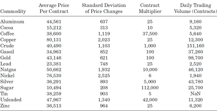
We consider 15 different liquid commodity futures, which do not have tight restrictions on the size of daily price moves (limit up/down). In particular, as
seen in TableI, we collect data on Aluminum, Copper, Nickel, Zinc, Lead, and
Table I
Summary Statistics
For each commodity used in our empirical study, the first column reports the average price per contract in U.S. dollars over our sample period January 1, 1996 to January 23, 2009. For instance, since the average gold price is $431.46 per ounce, the average price per contract is $43,146 since each contract is for 100 ounces. Each contract’s multiplier (100 in the case of gold) is reported in the third column. The second column reports the standard deviation of price changes. The fourth column reports the average daily trading volume per contract, estimated as the average daily volume of the most liquid contract traded electronically and outright (i.e., not including calendar-spread trades) in December 2010.
Average Price Standard Deviation Contract Daily Trading Commodity Per Contract of Price Changes Multiplier Volume (Contracts)
Aluminum 44,561 637 25 9,160
Cocoa 15,212 313 10 5,320
Coffee 38,600 1,119 37,500 5,640
Copper 80,131 2,023 25 12,300
Crude 40,490 1,103 1,000 151,160
Gasoil 34,963 852 100 37,260
Gold 43,146 621 100 98,700
Lead 23,381 748 25 2,520
Natgas 50,662 1,932 10,000 46,120
Nickel 76,530 2,525 6 1,940
Silver 36,291 893 5,000 43,780
Sugar 10,494 208 112,000 25,700
Tin 38,259 903 5 NaN
Unleaded 47,967 1,340 42,000 11,320
Zinc 36,513 964 25 6,200
York Commodities Exchange (COMEX); and Coffee, Cocoa, and Sugar from the New York Board of Trade (NYBOT). (Note that we exclude futures on various agriculture and livestock that have tight price limits.) We consider the sample period January 1, 1996 to January 23, 2009, for which we have data on all the
above commodities.10
For each commodity and each day, we collect the futures price measured in U.S. dollars per contract. For instance, if the gold price is $1,000 per ounce,
the price per contract is $100,000, since each contract is for 100 ounces. TableI
provides summary statistics on each contract’s average price, the standard deviation of price changes, the contract multiplier (for example, 100 ounces per contract in the case of gold), and daily trading volume.
We use the most liquid futures contract of all maturities available. By always using data on the most liquid futures, we are implicitly assuming that the trader’s position is always held in these contracts. Hence, we are assuming that when the most liquid futures contract nears maturity and the next contract becomes more liquid, the trader “rolls” into the next contract, that is, replaces
10Our return predictors use moving averages of price data lagged up to 5 years, which are
the position in the near contract with the same position in the far contract. Given that rolling does not change a trader’s net exposure, it is reasonable to abstract from the transaction costs associated with rolling. (Traders in the real world do in fact behave in this fashion. There is a separate roll market, which entails far smaller costs than independently selling the “old” contract and buying the “new” one.) When we compute price changes, we always compute the change in the price of a given contract (not the difference between the new contract and the old one), since this corresponds to an implementable return. Finally, we collect data on the average daily trading volume per contract as seen
in the last column of TableI. Specifically, we obtain an estimate of the average
daily volume of the most liquid contract traded electronically and outright (that is, not including calendar-spread trades) in December 2010 from an asset manager based on underlying data from Reuters.
B. Predicting Returns and Other Parameter Estimates
We use the characteristic-based model described in Example2in SectionV,
where each commodity characteristic is its own past return at various horizons. Hence, to predict returns, we run a pooled panel regression:
rts+1=0.001+ 10.32 f5D,s
t +122.34 ft1Y,s−205.59 ft5Y,s+ ust+1,
(0.17) (2.22) (2.82) (−1.79) (31)
where the left-hand side is the daily commodity price changes and the
right-hand side contains the return predictors: f5Dis the average past 5 days’ price
change divided by the past 5 days’ standard deviation of daily price changes,
f1Y is the past year’s average daily price change divided by the past year’s
standard deviation, and f5Y is the analogous quantity for a 5-year window.
Hence, the predictors are rolling Sharpe ratios over three different horizons; to avoid dividing by a number close to zero, the standard deviations are winsorized
below the 10th percentile of standard deviations. We estimate the regression
using feasible generalized least squares and report thet-statistics in brackets.
We see that price changes show continuation at short and medium
frequen-cies and reversal over long horizons.11The goal is to see how an investor could
optimally trade on this information, taking transaction costs into account. Of course, these (in-sample) regression results are only available now and a more realistic analysis would consider rolling out-of-sample regressions. However, using the in-sample regression allows us to focus on the economic insights un-derlying our novel portfolio optimization. Indeed, the in-sample analysis allows us to focus on the benefits of giving more weight to signals with slower alpha
11Erb and Harvey (2006) document 12-month momentum in commodity futures prices. Asness,
decay, without the added noise in the predictive power of the signals arising when using out-of-sample return forecasts.
The return predictors are chosen so that they have very different mean-reversion:
ft5D+1,s= −0.2519f5D,s t +ε5D
,s t+1
ft1Y+1,s= −0.0034f1Y,s t +ε
1Y,s
t+1 (32)
ft+5Y1,s= −0.0010f5Y,s t +ε
5Y,s t+1.
These mean-reversion rates correspond to a 2.4-day half-life for the 5-day sig-nal, a 206-day half-life for the 1-year sigsig-nal, and a 700-day half-life for the
5-year signal.12
We estimate the variance–covariance matrix using daily price changes
over the full sample, shrinking the correlations 50% toward zero. We set the
absolute risk aversion toγ =10−9, which we can think of as corresponding to
a relative risk aversion of one for an agent with $1 billion under management.
We set the time discount rate toρ =1−exp(−0.02/260), corresponding to a
2% annualized rate.
Finally, to choose the transaction cost matrix, we make use of price impact
estimates from the literature. In particular, we use the estimate from Engle,
Ferstenberg, and Russell (2008) that trades amounting to 1.59% of the daily
volume in a stock have a price impact of about 0.10%. (Breen, Hodrick, and
Korajczyk (2002) provide a similar estimate.) Furthermore, Greenwood (2005)
finds evidence that a market impact in one security spills over to other
secu-rities using the specification=λ, where we recall that is the variance–
covariance matrix. We calibrateas the empirical variance–covariance matrix
of price changes, where the covariance is shrunk 50% toward zero for robust-ness.
We choose the scalarλbased on the Engle, Ferstenberg, and Russell (2008)
estimate by calibrating it for each commodity and then computing the mean and median across commodities. Specifically, we collect data on the trading
volume of each commodity contract as seen in the last column of TableIand
then calibrateλfor each commodity as follows. Consider, for instance, unleaded
gasoline. Since gasoline has a turnover of 11,320 contracts per day and a daily price change volatility of $1,340, the transaction cost per contract when one
trades 1.59% of daily volume is 1.59%×11,320×λGasoline/2×1,3402, which is
0.10% of the average price per contract of $48,000 ifλGasoline=3×10⁻⁷.
We calibrate the trading costs for the other commodities similarly, and obtain
a median value of 5.0×10⁻⁷and a mean of 8.4
×10−7. There are significant
dif-ferences across commodities (for example, the standard deviation is 1.0×10⁻⁶),
reflecting the fact that these estimates are based on turnover while the
specifi-cation=λassumes that transaction costs depend on variances. While our
model is general enough to handle transaction costs that depend on turnover
12The half-life is the time it is expected to take for half the signal to disappear. It is computed
(for example, by using these calibratedλ’s in the diagonal of thematrix), we also need to estimate the spillover effects (that is, the off-diagonal elements).
Since Greenwood (2005) provides the only estimate of these transaction cost
spillovers in the literature using the assumption=λ, and since real-world
transaction costs likely depend on variance as well as turnover, we stick to
this specification and calibrateλas the median across the estimates for each
commodity. Naturally, other specifications of the transaction cost matrix would give slightly different results, but our main purpose is simply to illustrate the economic insights that we have proved theoretically.
We also consider a more conservative transaction cost estimate of λ=
10×10−7. This more conservative analysis can be interpreted as providing
the trading strategy of a larger investor (that is, we could equivalently reduce
the absolute risk aversionγ).
C. Dynamic Portfolio Selection with Trading Costs
We consider three different trading strategies: the optimal trading strategy
given by equation(27)(“optimal”), the optimal trading strategy in the absence
of transaction costs (“Markowitz”), and a number of trading strategies based on
static (i.e., one-period) transaction cost optimization as in equation(29)(“static
optimization”). The static portfolio optimization results in trading partially toward the Markowitz portfolio (as opposed to an aim portfolio that depends on signals’ alpha decays), and we consider 10 different trading speeds as seen
in Table II. Hence, under the static optimization, the updated portfolio is a
weighted average of the Markowitz portfolio (with weight denoted “weight on Markowitz”) and the current portfolio.
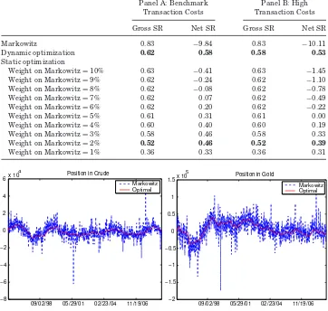
Table II reports the performance of each strategy as measured by,
respec-tively, its gross Sharpe ratio and its net Sharpe ratio (i.e., its Sharpe ratio after accounting for transaction costs). Panel A reports these numbers using our base-case transaction cost estimate (discussed earlier), while Panel B uses our high transaction cost estimate. We see that, naturally, the highest Sharpe ratio before transaction costs is achieved by the Markowitz strategy. The op-timal and static portfolios have similar drops in gross Sharpe ratio due to their slower trading. After transaction costs, however, the optimal portfolio is the best, significantly better than the best possible static strategy, and the Markowitz strategy incurs enormous trading costs.
It is interesting to consider the driver of the superior performance of the optimal dynamic trading strategy relative to the best possible static strategy. The key to the outperformance is that the dynamic strategy gives less weight to the 5-day signal because of its fast alpha decay. The static strategy simply tries to control the overall trading speed, but this is not sufficient: it either incurs large trading costs due to its “fleeting” target (because of the significant reliance on the 5-day signal), or trades so slowly that it is difficult to capture the return. The dynamic strategy overcomes this problem by trading somewhat fast, but trading mainly according to the more persistent signals.
To illustrate the difference in the positions of the different strategies, Figure3
Table II
Performance of Trading Strategies before and after Transaction Costs
This table shows the annualized Sharpe ratio gross (“Gross SR”) and net (“Net SR”) of trading costs for the optimal trading strategy in the absence of trading costs (“Markowitz”), our optimal dynamic strategy (“Dynamic”), and a strategy that optimizes a static one-period problem with trading costs (“Static”). Panel A illustrates these results for a low transaction cost parameter, while Panel B uses a high one. We highlight in bold the performance of our dynamic strategy (which has the highest net SR among all strategies considered) and that of the static strategy with the highest net SR among the static ones.
Panel A: Benchmark Panel B: High Transaction Costs Transaction Costs
Gross SR Net SR Gross SR Net SR
Markowitz 0.83 −9.84 0.83 −10.11
Dynamic optimization 0.62 0.58 0.58 0.53
Static optimization
Weight on Markowitz=10% 0.63 −0.41 0.63 −1.45
Weight on Markowitz=9% 0.62 −0.24 0.62 −1.10
Weight on Markowitz=8% 0.62 −0.08 0.62 −0.78
Weight on Markowitz=7% 0.62 0.07 0.62 −0.49
Weight on Markowitz=6% 0.62 0.20 0.62 −0.22
Weight on Markowitz=5% 0.61 0.31 0.61 0.00
Weight on Markowitz=4% 0.60 0.40 0.60 0.19
Weight on Markowitz=3% 0.58 0.46 0.58 0.33
Weight on Markowitz=2% 0.52 0.46 0.52 0.39
Weight on Markowitz=1% 0.36 0.33 0.36 0.31
09/02/98 05/29/01 02/23/04 11/19/06
Figure 3. Positions in crude and gold futures.This figure shows the positions in crude and gold for the optimal trading strategy in the absence of trading costs (“Markowitz”) and our optimal dynamic strategy (“Optimal”).
0 10 20 30 40 50 60 70
4 Optimal Trading after Shock to Signal 1 (5−Day Returns)
Markowitz
5 Optimal Trading after Shock to Signal 2 (1−Year Returns)
Markowitz
5 Optimal Trading after Shock to Signal 3 (5−Year Returns)
Markowitz Optimal Optimal (high TC)
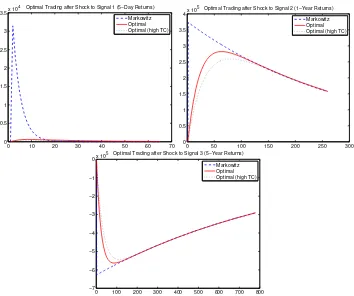
Figure 4. Optimal trading in response to shocks to return-predicting signals.This figure shows the response in the optimal position following a shock to a return predictor as a function of the number of days since the shock. The top left panel considers a shock to the fast 5-day return predictor, the top right panel considers a shock to the 1-year return predictor, and the bottom panel to the 5-year predictor. In each case, we consider the response of the optimal trading strategy in the absence of trading costs (“Markowitz”) and our optimal dynamic strategy (“Optimal”) using high and low transactions costs.
portfolio is short, and larger when the expected return is large, but moderates the speed and magnitude of trades.
D. Response to New Information
It is instructive to trace the response to a shock to the return predictors,
namely, toεit,sin equation(32). Figure4shows the responses to shocks to each
return-predicting factor, namely, the 5-day factor, the 1-year factor, and the 5-year factor.
slowly out of the position as the alpha decays, the lines cross as the optimal strategy eventually has a larger position than the Markowitz strategy.
The second panel shows the response to the 1-year factor. The Markowitz strategy jumps up and decays, whereas the optimal position increases more smoothly and catches up as the Markowitz strategy starts to decay. The third panel shows the same for the 5-year signal, except that the effects are slower and with opposite sign, since 5-year returns predict future reversals.
VII. Conclusion
This paper provides a highly tractable framework for studying optimal trad-ing strategies in the presence of several return predictors, risk and correlation considerations, as well as transaction costs. We derive an explicit closed-form solution for the optimal trading policy, which gives rise to several intuitive results. The optimal portfolio tracks an aim portfolio, which is analogous to the optimal portfolio in the absence of trading costs in its trade-off between risk and return, but is different since more persistent return predictors are weighted more heavily relative to return predictors with faster alpha decay. The optimal strategy is not to trade all the way to the aim portfolio, since this entails excessively high transaction costs. Instead, it is optimal to take a smoother and more conservative portfolio that moves in the direction of the aim portfolio while limiting turnover.
Our framework constitutes a powerful tool to optimally combine various re-turn predictors taking into account their evolution over time, decay rate, and correlation, and trading off their benefits against risks and transaction costs. Such dynamic trade-offs are at the heart of the decisions of “arbitrageurs” that help make markets efficient as per the efficient market hypothesis. Ar-bitrageurs’ ability to do so is limited, however, by transaction costs, and our model provides a tractable and flexible framework for the study of the dynamic implications of this limitation.
We implement our optimal trading strategy for commodity futures. Naturally, the optimal trading strategy in the absence of transaction costs has a larger Sharpe ratio gross of fees than our trading policy. However, net of trading costs our strategy performs significantly better, since it incurs far lower trading costs while still capturing much of the return predictability and diversification benefits. Furthermore, the optimal dynamic strategy is significantly better than the best static strategy, that is, taking dynamics into account significantly improves performance.
In conclusion, we provide a tractable solution to the dynamic trading strategy in a relevant and general setting that we believe to have many interesting applications. The main insights for portfolio selection can be summarized by the rules that one should aim in front of the target and trade partially toward the current aim.
Appendix A: Proofs
In what follows we make repeated use of the notation
¯
Assuming that the value function is of the posited form, we calculate the expected future value function as
Et[V(xt, ft+1)]= −
The agent maximizes the quadratic objective−12x⊤
t Jtxt+xt⊤jt+dtwith
The maximum value is attained by
xt =Jt−1jt, (A6)
which is equal to V(xt−1,ft)=12jt⊤Jt−1jt+dt. Combining this fact with (6)we
obtain an equation that must hold for allxt−1and ft, which implies the following
restrictions on the coefficient matrices:13
−ρ¯−1Axx=¯(γ +¯ +Axx)−1¯ −,¯ (A7)
The existence of a solution to this system of Riccati equations can be
estab-lished using standard results, for example, as in Ljungqvist and Sargent (2004).
In this case, however, we can derive explicit expressions as follows. We start by lettingZ=¯−12Axx¯−12 andM=¯−12¯−12, and rewriting equation(A7)as
¯
ρ−1Z= I−(γM+I+Z)−1, (A10)
13Remember thatA
which is a quadratic with an explicit solution. Since all solutions Z can be
written as a limit of polynomials of the matrixM, we see thatZandMcommute
and the quadratic can be sequentially rewritten as
Z2+Z(I+γM−ρ¯I)=ργ¯ M, (A11)
Note that the positive-definite choice of solutionZis the only one that results
in a positive-definite matrix Axx.
The other value function coefficient determining optimal trading is Ax f,
which solves the linear equation(A8). To write the solution explicitly, we note
first that, from(A7),
¯
Finally, Af f is calculated from the linear equation(A9), which is of the form
¯
ρ−1Af f =Q+(I−)⊤Af f(I−) (A19)
with
Q=(B+Ax f(I−))⊤(γ +¯ +Axx)−1(B+Ax f(I−)), (A20)
The solution is easiest to write explicitly for diagonal, in which case
Af f,i j =
¯
ρQi j
1−ρ¯(1−ii)(1−j j)
. (A21)
In general,
vecAf f
=ρ¯I−ρ¯(I−)⊤⊗(I−)⊤−1vec(Q). (A22)
One way to see that Af f is positive-definite is to iterate (A19) starting with
A0f f =0.
We conclude that the posited value function satisfies the Bellman
equation. Q.E.D.
Proof of Proposition2
Differentiating the Bellman equation(5)with respect toxt−1gives
−Axxxt−1+Ax fft=(xt−xt−1),
which clearly implies(7)and(8).
In the case=λfor some scalarλ >0, the solution to the value function
coefficients is Axx =a, whereasolves a simplified version of(A7):
−ρ¯−1a= λ¯
2
γ+λ¯+a−λ,¯ (A23)
or
a2+(γ+λρ¯ )a−λγ =0, (A24)
with solution
a= (γ+λρ¯ )
2+4γ λ−(γ+λρ¯ )
2 . (A25)
It follows immediately that−1A
xx=a/λ.
Note thatais symmetric in (λρ(1−ρ)−1, γ). Consequently,aincreases inλif
and only if it increases inγ. Differentiating(A25)with respect toλ, one gets
2da
dλ = −ρ¯ −1ρ
+12
(2(γ+λρ¯ )+4γ)
√
(γ+λρ¯ )2+4γ λ. (A26)
This expression is positive if and only if
¯
ρ−2ρ2(γ +λρ¯ )2+4γ λ≤(γ+λρ¯ ) ¯ρ−1ρ+2γ2, (A27)
Finally, note thata/λis increasing inγ and homogeneous of degree zero in
(λ, γ), so that applying Euler’s theorem for homogeneous functions gives
d dλ
a
λ = −
d dγ
a
λ <0. (A28)
Q.E.D.
Proof of Proposition3
We show that
aimt=(γ +Axx)−1
γ ×Markowitzt+Axx×Et(aimt+1) (A29)
by using(8),(A8), and(A7)successively to write
aimt=A−xx1Ax f ft (A30)
=A−xx1γ +¯ +Axx
−1
γ ×Markowitzt+Axx×Et(aimt+1)
=(γ +Axx)−1
γ ×Markowitzt+Axx×Et(aimt+1).
To obtain the last equality, rewrite(A7)as
(−Axx)−1(γ +¯ +Axx)=¯ (A31)
and then further
γ +Axx =(γ +¯ +Axx)−1Axx, (A32)
since Axx−1=−1Axxbecause, as discussed in the proof of Proposition 1,
MZ=ZM. Equation(12)follows immediately as a special case.
For part (ii), we iterate(A29)forward to obtain
aimt =(γ +Axx)−1×
∞
τ=t
Axx(γ +Axx)−1
(τ−t)
γ ×Et(Markowitzτ),
which specializes to(13). Given that aincreases in λ, z decreases in λ.
Fur-thermore,zincreases inγ if and only ifa/γ decreases, which is equivalent (by
symmetry) toa/λdecreasing inλ. Q.E.D.
Proof of Proposition4
In the case=λ, equation(A8)is solved by
Ax f =λB((γ+λ¯+a)I−λ(I−))−1
=λB((γ+λρ¯ +a)I+λ)−1
= Bγ a+
−1
where the last equality follows from (A24) by dividing across byλaand rear-ranging. The aim portfolio is
aimt=(a)−1B
γ
a+
−1
ft, (A34)
which is the same as(14). Equation(15)is immediate.
For part (iii), we use the result shown above (proof of Proposition 2) that
a increases in λ, which implies that (1+φja/γ)/(1+φia/γ) does whenever
φj > φi. Q.E.D.
Proof of Proposition5
Rewriting(7)as
xt =(I−−1Axx)xt−1+−1Axx×aimt (A35)
and iterating this relation backwards gives
xt=
The conjectured value function is
1 2Et
˜
ε⊤t+1Ayyε˜t+1+A0.
The trader consequently choosesxtto solve
max
which is a quadratic of the form−1
2x⊤Jx+x⊤jt+dt, with
The value ofxattaining the maximum is given by
xt= J−1jt, (A49)
and the maximal value is
The unknown matrices have to satisfy a system of equations encoding the
equality of all coefficients in(A51). Thus,
−ρ¯−1Axx =Sx⊤J−1Sx−¯ −ρ¯−1C+C˜⊤AyyC,˜ (A52)
¯
ρ−1Axy=Sx⊤J−1Sy−C˜⊤Ayy(I−), (A53)
¯
ρ−1Ayy=S⊤yJ−1Sy+(I−)⊤Ayy(I−). (A54)
For our purposes, the more interesting observation is that the optimal
posi-tionxtis rewritten as
xt=xt−1+I−J−1Sx
Acharya, Viral, and Lasse Heje Pedersen, 2005, Asset pricing with liquidity risk,Journal of Fi-nancial Economics77, 375–410.
Almgren, Robert, and Neil Chriss, 2000, Optimal execution of portfolio transactions,Journal of Risk3, 5–39.
Amihud, Yakov, and Haim Mendelson, 1986, Asset pricing and the bid-ask spread,Journal of Financial Economics17, 223–249.
Asness, Cliff, Tobias Moskowitz, and Lasse Heje Pedersen, 2013, Value and momentum everywhere,
Journal of Finance68, 929–985.
Balduzzi, Pierluigi, and Anthony W. Lynch, 1999, Transaction costs and predictability: Some utility cost calculations,Journal of Financial Economics52, 47–78.
Bertsimas, Dimitris, and Andrew W. Lo, 1998, Optimal control of execution costs, Journal of Financial Markets1, 1–50.
Breen, William J., Laurie S. Hodrick, and Robert A. Korajczyk, 2002, Predicting equity liquidity, Management Science48, 470–483.
Brunnermeier, Markus K., and Lasse H. Pedersen, 2005, Predatory trading,Journal of Finance 60, 1825–1863.
Campbell, John Y., and Luis M. Viceira, 2002,Strategic Asset Allocation Portfolio Choice for Long-Term Investors(Oxford University Press, Oxford, UK).
Carlin, Bruce I., Miguel Lobo, and S. Viswanathan, 2008, Episodic liquidity crises: Cooperative and predatory trading,Journal of Finance62, 2235–2274.
Constantinides, George M., 1986, Capital market equilibrium with transaction costs,Journal of Political Economy94, 842–862.
Davis, M., and A. Norman, 1990, Portfolio selection with transaction costs,Mathematics of Oper-ations Research15, 676–713.
Engle, Robert, and Robert Ferstenberg, 2007, Execution risk,Journal of Portfolio Management33, 34–45.
Engle, Robert, Robert Ferstenberg, and Jeffrey Russell, 2008, Measuring and modeling execution cost and risk, Working paper, University of Chicago.
Erb, Claude, and Campbell R. Harvey, 2006, The strategic and tactical value of commodity futures, Financial Analysts Journal62, 69–97.
G ˆarleanu, Nicolae, 2009, Portfolio choice and pricing in imperfect markets,Journal of Economic
Theory144, 532–564.