Keywords—ODEs, 10 th order IRK method, numerical technique,

(1)

DOI:10.23960/ins.v1i1.11 Published online: 01/10/2016



Abstract—To construct a scheme of implicit Runge-Kutta methods, there are a number of coefficients that must be determined and satisfying consistency properties and Butcher’s simplifying assumptions. In this paper we provide the numerical simulation technique to obtain a scheme of 10th _{order Implicit Runge-Kutta} (IRK10) method. For simulation process, we construct an algorithm to compute all the coefficients involved in the IRK10scheme. The algorithm is implemented in a language programming (Turbo Pascal) to obtain all the required coefficients in the scheme. To show that our scheme works correctly, we use the scheme to solve Hénon-Heiles system.

Keywords—ODEs, 10thorder IRK method, numerical technique, Hénon-Heiles system

I. INTRODUCTION

et a first order ordinary differential equation system (ODES)

In (1), where the “prime“indicates differentiation with

respect to x, y is a D-dimensional vector



y



D



, and

D D

x

f

:







. The ODES (1)-(2) is the well-known

the first order of initial value problem. To solve problem (1)-(2) can be used analytical and/or numerical procedures. But, for solving the special problems (Hamiltonian and Divergen Free systems, for examples) and taking efficiency and effective calculations, some mathematicians recommended to use numerical approximations ([1-4,5]). One of numerical methods which can be used to solve (1-2) which is enough recognized and a lot of used is Runge-Kutta method.

Definition : Let

b

_i

,

a

_ij

,

and

c

_i



i

,

j

_

1 ,

2 ,



,

s



_{be real}

1_{Department of Mathematics, Faculty of Mathematics and Natural}

Sciences, University of Riau, Kampus Bina Widya Simpang Baru Km. 12.5 Pekanbaru, Riau, Indonesia.

2_{Department of Mathematics, Faculty of Mathematics and Natural}

Sciences, University of Lampung, Soemantri Brojonegoro 1 Bandar Lampung, Lampung, Indonesia.

*_{Correspondence to 2}nd_{Author, email: lazakaria.1969@fmipa.unila.ac.id.} Tel.:+62-721-704625; fax: +62-721-704625.

is called ans-stageRunge-Kutta method. When

a

_ij



0

for

j

i



the method is called anexplicit Runge-Kuttamethod.

Ifaij= 0

i



j

and least oneaii0, the method is called a

diagonal implicit Runge-Kutta method. If all of the diagonal elements are identical, aij =  for i = 1,2,...,s, the

method is called a singly diagonal implicit Runge-Kutta

method. In all other cases, the method is called an implicit Runge-Kutta method. The Runge-Kutta methods are often given in the form of a tableau containing their coefficients

Consistency in the Runge-Kutta methods is investigated

by using a Taylor series expansion. Anys-stage Runge-Kutta

process of the form (3) or (4) is consistent if method to haveasymptotic behavior

O

 

τ

.

There are some advantages to use Implicit Runge-Kutta (IRK) methods (see [6-8]). (1) IRK methods usually are required for systems whose solutions contain rapidly decaying components (see [6]); (2) Some methods may also

be used in preserving the symplectic structure of

Hamiltonian systems; (3) IRK methods (Gauss quadratures)

have a number of big potency for the computing of integrate the geometry; (4) high order integrator to be used by the reason of doubled accuracy is recommended; (5) to evaluate the vector field "costly", all stage-sin IRK can be evaluated by parallel and; (6) IRK can be solve the ordinary differential equation (ODE) or system (ODEs) in general.

To construct a scheme of IRK methods, Butcher discovered the existence of s-stage methods of order 2s,for

alls. He usedsimplifying assumptionsto find these methods.

The simplifying assumptions are

The Scheme of 10

th

_{Order Implicit Runge-Kutta Method to Solve the First Order}

of Initial Value Problems

Z. Bahri

1

_{, L. Zakaria}

2,*

_{, Syamsudhuha}

1

(2)

 

1

Based on consistency property and Butcher’s simplifying

assumptions, Hairer et.al (2007)[7] and Ismail (2009)[8]

derive some IRK methods new analytical procedures.

In analytical procedure, we can use the idea of collocation to derive IRK methods ([4],[8]). Unfortunately, for the stage ofstage s≥ 3, constructing an integrator IRK using analytical

procedure will be difficult because there are some values of

, , and ( , 1, 2,..., )

i i ij

b c a i j s must be determined.

Therefore, the numerical technique or procedure is an alternative choice to use. In this procedure, we can use computer to determine the values of

c

i

(

i



1, 2,..., )

s

,

and

i ij

b a

( ,

i j



1, 2,..., )

s

.

Notice that one important property of IRK method is symplecticness. An IRK method (4) is symplectic if it satisfy the following condition ([9])

0 , ,

{1, 2,..., }

i j i ij j ji

b b



b a



b a



i j



s

.

II. RESULT ANDDISCUSSION

In this section, we describe how to get a class of 10th_order

IRK method using computer simulation to obtain all

Butcher’s coefficient values (4) based on Butcher’s

simplifying assumptions (5).

Setting

k

   

i

j

s

1, 2, 3, 4, 5

into first equation in (5), we have the following systems

11 12 13 14 15 1

Then, from second equation in (5) we have the following systems

Equations (6.1)-(10.5) solved respect to with

(3)



_{c (-3c +30c c c + 5c (c +c + c ) -10c (c c +c (c +c )))}2 3 2



pseudo codeas below :

Determining_The_Butcher_Coefficients_10th_{_order_IRK}

{Name of Algorithm}

{This algorithm is used to the determination simulation assess

the Butcher’s coefficients for the 10th _{order IRK method with}

the choice assess 0ci 1,i 1, 2, 3, 4, 5 . at random}

the 10th_{order IRK method are obtained.}}

DECLARATION Label 10 I : integer

c1, c2, c3, c4, c5,b1,b2, b3,b4,b5,a11,a12,a13,a14 ,a15,a21,a22,a23,a24,a25,a31,a32,a33,a34,a35,a41 ,a42,a43,a44,a45,a51,a52,a53,a54,a55:real;

function f1(c1,c2,c3,c4,c5:real):real begin

f1← setting the rhs. Of equation 12.1 here

(4)

begin

RETURN (f3)

f4← setting the rhs. Of equation 12.4here RETURN (f4)

RETURN (f5)

DESCRIPTION BEGIN 10:

Randomize Repeat

c1← Random c2 ← Random

c3← Random c4 ← Random

c5← Random

until ((abs(c1+c2+c3+c4+c5–2.5) <= 0.0000001) and

(c1>0) and (c2>0) and (c3>0) and (c4>0) and (c5>0) and (c1<>c2) and (c2<>c3) and (c3<>c4) and (c4<>c5) )

b1← f1(c1,c2,c3,c4,c5) b2 ← f2(c1,c2,c3,c4,c5)

b3← f3(c1,c2,c3,c4,c5) b4← f4(c1,c2,c3,c4,c5)

b5← f4(c1,c2,c3,c4,c5)

if ( ((abs(b1+b2+b3+b4+b5 - 1 ) > 0.0000001) or (b1<0) or (b2<0) or (b3<0) or (b4<0) or (b5<0)) ) then goto 10 else

BEGIN

a11← setting the rhs. Of equation 13.1 here

a12← setting the rhs. Of equation 13.2 here a13← setting the rhs. Of equation 13.3 here

a31← setting the rhs. Of equation 15.1 here a32← setting the rhs. Of equation 15.2 here

BEGIN

Write(c1, c2, c3, c4, c5,b1,b2, b3,b4,b5,

,a11,a12,a13,a14,a15,a21,a22,a23,a24,a25 ,a31,a32,a33,a34,a35,a41,a42,a43,a44,a45 ,a51,a52,a53,a54,a55)

end END.

Implementing the algorithm to TURBO PASCAL

programming, we have a the 10th _{order of implicit}

Runge-Kutta methods that given in the form of a tableau containing their coefficients below

Table 1.The Butcher’s coefficients for the 10th _{order IRK}

0.00062327669 0.62262155069 0.68561704247 0.30589831341 0.88523974386

0.00063421625 0.00001105145 -0.00000999963 0.00000344788 0.00000094280 0.09617192074 -0.08577858789 0.19691976268 0.44098804083 -0.02567958566 0.09620099283 -0.05393518544 0.22869146117 0.44069256651 -0.02603279259 0.10069140845 -0.57368596565 0.50477982176 0.31903127918 -0.04491823033 0.09527844353 -0.20783782461 0.51158700582 0.44878101607 0.03743110305

III. NUMERICALEXPERIMENT

In this section, we present an application of our scheme to solve Henon-Heiles problem. The Hénon-Heiles problem is typically non integrable system and have simultaneously and quasi periodic solutions. The Hénon-Heiles system is defined by (see [8])



2 2





2 2

 

2



2

1 2 1 2 1 2 2

1 1 1

, ,

-2 2 3

H T V T p p V q q  q q q (18)

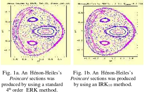
We apply the 10th _{order IRK method (}_IRK₁₀_{) to solve}

problem (18). The results of usingIRK10is displayed in the

figure 1b. To show them, we usedMATHEMATICA.

The figures displayed arePoincarésections (i.e. sections

of various orbits), for an energyEand time-stepsτ. To obtain ourPoincarésections, we use the idea of linear interpolation [10]. The Poincaré sections is the integration results as points of intersection of the flow with the

q

₁



0

-plane. Here we set 62 initial points.

In all graphs, the blue dots indicate that the points are

moving up to

q

₁



0

-plane whereas the red dots indicate that

the points are moving down the plane. Fig. 1.b shows that the

scheme of 10th _{IRK method can be used to solve}

Hénon-Heiles problem (18).

In Fig. 1.a and Fig. 1.b, we show a poincaré section for

Hénon-Heiles (18) using the 10th _{order IRK method whose}

tableau are given in Table.1 and a standard 4th_{order explicit}

Runge-Kutta methods, respectively. We set an energy

E=1.25,τ= 0.01, and the number of iterations = 100,000 for

(5)

Fig. 1a. An Hénon-Heiles’s Poincarésections was produced by using a standard

4th_{order ERK method.}

Fig. 1b. An Hénon-Heiles’s Poincarésections was produced

by using an IRK10method.

IV. CONCLUSION

Based on theoretical surveying, algorithm designing and implementing, and numerical problem solving before, we

conclude that we can construct a scheme of 10th_{order of IRK}

methods via simulating to choose ci (i 1..5) values that

satisfy 5

1

1 = 2

2

s i i

c 





,

5

1 =1 i i

b





, and 5

1

, 1 ..5

i ij

j

c a i





 .

Although, we have not exact values for

c b

_i

,

_i

,

and

, ( , 1, 2, 3.4) ij

a i j , but our schemes can solve a problem

of the first order of ordinary differential equation system like classical methods (Gauss-Legendre for example).

ACKNOWLEDGMENT

The first authors sincerely wish to acknowledge the continuing help, advice, and influence of the second and the third authors. They are constantly interest and enthusiasm in all parts of this paper. Thanks are also due to Riau University (staff and service employees) through Computer Laboratory FMIPA UR for funding and servicing all of our research needs. Finally, we thanks to our family for their moral support. We are deeply indebted to them for this.

REFERENCES

[1] L. Zakaria, “A Numerical Technique to Obatain Scheme of 8th_Order Implicit Runge-Kutta Method to Solve the First Order of Initial Value

Problems,” inProceeding of IndoMS International Conference on Mathematics and Applications(IICMA), Yogyakarta, 2009, pp 425-434

[2] G. R W. Quispel and C. Dyt, “Volume-preserving integrators have

linear error growth,”Physics Letters A.242,1998, 25-30.

[3] J.M. Sanz-Serna and M.P. Calvo,Numerical Hamiltonian Problems, Chapman & Hall, New York, 1994, pp. 27-54

[4] G.S. Turner, “Three-Dimensional Reversible Mappings,” Ph.D. dissertation, Dept. Math., La Trobe Univ., Australia. 1994

[5] L. Zakaria, “Applying Linear Interpolating To Show Poincaré Section

of The Hénon-Heiles,” Mathematics and Its Learning Journal.

Special Edition, Malang State University, 2002, 1003-1008. [6] J.C. Butcher, The Numerical Analysis of Ordinary Differential

Equations.Wiley, New York, 1987, pp 51-316

[7] E. Hairer, R.I. McLachlan, and A. Razakarivony, “Achieving Brouwer’s law with implicit Runge–Kutta methods,” Research

Report, 2007

[8] F. Ismail, “Sixth Order Singly Diagonally Implicit Runge-Kutta Nyström Method with Explicit First Stage for Solving Second Order

Ordinary Differential Equations,” European Journal of Scientific Research,26, 470-479, 2009.

[9] H. Yoshida, “Construction of higher order symplectic integrators,” Physics Letters A.150, 1990, 262-268.