Inverse Stochastic Linear Programming
G¨orkem Saka ∗, Andrew J. Schaefer
Department of Industrial Engineering University of Pittsburgh Pittsburgh, PA USA 15261
Lewis Ntaimo
Department of Industrial and Systems Engineering Texas A&M University
College Station, TX USA 77843
Abstract
Inverse optimization perturbs objective function to make an initial feasible solution optimal with respect to perturbed objective function while minimizing cost of perturbation. We extend inverse optimization to two-stage stochastic linear programs. Since the resulting model grows with number of scenarios, we present two decomposition approaches for solving these problems.
1
Introduction
An inverse optimization problem infers the values of the objective coefficients, given the values of optimal decision variables. The aim of inverse optimization is to perturb the objective vector from
c tod so that an initial feasible solution ˆx with respect to objective vector c becomes an optimal solution with respect to perturbed objective vector dand the “cost of perturbation” is minimized. Inverse optimization has many application areas, and inverse problems have been studied ex-tensively in the analysis of geophysical data [20, 21, 24, 25]. Recently, inverse optimization has extended into a variety of fields of study. Inverse optimization was applied in geophysical studies [5, 6], to predict the movements of earthquakes assuming that earthquakes move along shortest paths. Traffic equilibrium [11] is another application area where the minimum total toll is imposed to make the user equilibrium flow and system optimal flow equal. Inverse multicommodity flows were used in railroad scheduling to determine the arc costs based on a specific routing plan [10].
Another application of inverse optimization is the area of just-in-time scheduling. In this case the objective is to schedule the production so as to deviate, in each period, as little as possible from the target production quantity of each product [14]. In political gerrymandering the goal is to modify the current boundaries so as to achieve majority for a certain outcome while taking into account population numbers segmented as per various political options, and limitations on the geometry of the boundaries [7, 14].
Zhang and Liu [17] suggested a solution method for general inverse linear programs (LPs) including upper and lower bound constraints based on the optimality conditions for LPs. Their objective function was to minimize the cost of perturbation based on the L1 norm. Ahuja and
To consider the inverse optimization problem under the weighted L1 norm involves solving the
problem according to the objective MinP
j∈Jvj |dj−cj |, where J is the variable index set, dj
and cj are the perturbed and original objective cost coefficients, respectively, and vj is the weight
coefficient. By introducing variablesαj and βj for each variablej∈J, this objective is equivalent
to the following problem: Min X
j∈J
vj(αj+βj)
s.t. dj−cj =αj−βj, j ∈J,
αj ≥0, βj ≥0, j ∈J.
Two-stage stochastic linear programming (2SSLP) [3, 4, 8] considers LPs in which some problem data are random. In this case, “first-stage” decisions are made without full information on the random events while “second-stage” decisions (or corrective actions) are taken after full information on the random variables becomes available. This paper extends deterministic inverse LP to 2SSLP and provides preliminary computational results. Although many of the applications of inverse optimization are stochastic in nature, to the best of our knowledge, deterministic versions of these problems have been considered so far. With this paper, we add this stochastic nature to inverse problems.
In the next section, we formally characterize feasible cost vectors for inverse 2SSLP. In Section 3, we outline two large-scale decomposition techniques for solving inverse 2SSLPs. We conclude with computational results in Section 4.
2
Inverse Stochastic Linear Programming
of scenarios, Jk denotes the index set of second-stage variables for scenariok∈ K,Ik denotes the index set of second-stage constraints for scenario k∈ K. The 2SSLP in extensive form (EF) can be given as follows:
We associate first-stage constraints (1) with the dual variablesπi0, and second-stage constraints (2) with πik. Then the dual of EF can be given as follows:
LP optimality conditions require that at optimality, a primal solution (x,{yk}∀k∈K) is feasible
to (1)-(3), and a corresponding dual solution (π0,{πk}∀k∈K) is feasible to (4)-(6), and the following
complementary slackness (CS) conditions are satisfied:
Let B0 denote the set of binding constraints among the first-stage constraints (1) with respect to an initial primal feasible solution (ˆx,{yˆk}
∀k∈K), and letBk, k∈ Kbe the set of binding constraints
among the second-stage constraints (2). Then we can now rewrite the CS conditions as follows:
• πi0= 0 for all i∈I0\B0,
(qkj)′ and the primal-dual pair satisfies the CS conditions. Combining the dual feasibility condition with the newly constructed CS conditions gives the following characterization of inverse feasible cost vectors for 2SSLP:
Under the weightedL1 norm, the problem is
MinX denote the weight vectors associated with the first and second stage, respectively. In order to linearize this nonlinear objective we define α0j, βj0 and set dj −cj =α0j −βj0, where α0j ≥ 0 and
βj0 ≥0, ∀j∈J0. In the same manner, we defineαjk,βjkand set (qjk)′−qjk=αkj−βjk, whereαkj ≥0 and βk
The inverse 2SSLP under the weightedL1 norm is to minimize the first-stage weighted absolute
cost of perturbation plus the expected second-stage weighted absolute cost of perturbation. We formally state the inverse 2SSLP in EF as follows:
MinX
restate equations (10) and (11) as follows:
−α0j +β0j ≥cπj0, j ∈J0, (14)
−αkj +βjk≥cjπk, k∈ K, j ∈Jk. (15)
There are two sets of three mutually exclusive cases to consider:
• αkj = 0, βjk=cπjk ⇒(qjk)′ =qkj −cπjk
Case 5. cπjk <0
• αkj =βjk= 0⇒(qkj)′ =qjk
Case 6. cπjk = 0
• cπk
j = 0⇒αkj =βjk= 0⇒(qkj) ′
=qk j
3
Decomposition Approaches for Solving Inverse Stochastic
Lin-ear Programs
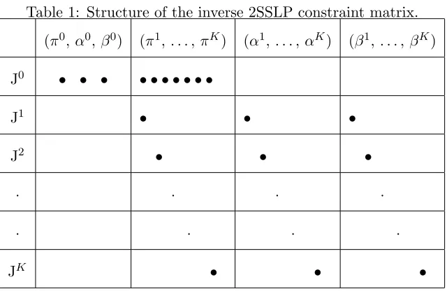
Unfortunately, the inverse 2SSLP problem (10) - (13) grows with the number of scenarios |K|. This leads us to consider decomposition approaches. Table 1 shows the rearranged constraints and variables in a matrix format where K = 1· · ·K which demonstrates the idea behind how the division between the constraints and variables has been made. For each set of variables, a dot appears if the variables in the set have nonzero coefficients. As can be seen in the table, the constraint setsJk, k∈ Khave a nice structure. So, we can setJ0 as the linking constraint set and a decomposition approach such as Dantzig-Wolfe decomposition [9] or Lagrangian relaxation [12] may be utilized. Furthermore, ({αk, βk}
∀k∈K) do not appear in J0 constraints and (π0, α0, β0) do not
appear inJk, k∈ Kconstraints. Therefore, the problem is relatively easy to solve when only these variables are present. So, ({πk}∀k∈K) are the linking variables for which Benders’ decomposition
[2] is appropriate.
3.1 Dantzig-Wolfe Decomposition of the Inverse Extensive Form
constraints as “easy” and “hard”. Rather than solving the LP with all the variables present, the variables are added as needed.
Table 1: Structure of the inverse 2SSLP constraint matrix. (π0,α0,β0) (π1,. . .,πK) (α1,. . .,αK) (β1,. . .,βK)
J0 • • • • • • • • • •
J1 • • •
J2 • • •
· · · ·
· · · ·
JK • • •
Observe that if one views the (π1,· · · , πK) variables as “first-stage” variables, the resulting inverse 2SSLP may be interpreted as a 2SSLP as well. Based on Table 1 Jk, k ∈ K decompose into a set of disjoint block constraints. So, for the inverse 2SSLP,Jk, k ∈ K are easy constraints
and J0 are hard constraints. Optimizing the subproblem by solving K independent LPs may be preferable to solving the entire system. Let (πk, αk, βk)1 · · · (πk, αk, βk)qk be the extreme points
and (πk, αk, βk)qk+1 · · · (πk, αk, βk)rk be the extreme rays ofPk. We can rewrite the points in the
problem:
In the above problem, constraints (16) are coupling constraints while constraints (17) are convexity rows. Note that problem (16) - (18) has fewer constraints than the original problem (10) - (13). However, since the points in the easy polyhedra are rewritten in terms of extreme points and extreme rays, the number of variables in the Dantzig-Wolfe master problem is typically much larger than in the original problem. Therefore a restricted master problem can be constructed with a very small subset (Λ(k)) of the columns in the full master problem as follows:
MinX
of the restricted master problem, so that thekth(k∈ K) subproblem takes the following form:
Min
X
j∈Jk
vjkpk(αkj +βjk)− X i∈Bk
tkijπki
uj−uk0 (22)
s.t. X
i∈Bk
wijkπik−pkαkj +pkβjk≥pkqjk, j ∈Jk, (23)
πki, αkj, βjk≥0, j ∈Jk. (24)
The Dantzig-Wolfe algorithm terminates when the optimum solution of the subproblem is greater than or equal to zero for all k ∈ K. Otherwise, the variable with the minimum reduced cost is added to the restricted master problem.
3.2 Benders’ Decomposition of the Inverse Extensive Form
In Benders’ decomposition [2], variables are divided into two sets as “easy” and “complicating” (linking) variables. The problem with only easy variables is relatively easy to solve. Benders’ decomposition projects out easy variables and then solves the remaining problem with linking variables. In this algorithm, easy variables are replaced with more constraints. The number of constraints is exponential in the number of easy variables. However, constraints are added on an as needed basis which overcomes the problem of an exponential number of constraints.
problem (10) - (13) is equivalent to:
Having written the equivalent problem (25)-(27) and associated optimal dual variables (u0j, ukj) with constraints (26)-(27) respectively, we can project out the easy variables to come up with the following Benders’ Master Problem (BMP):
Benders’ subproblem (BSP) for the inverse extensive form is solved:
If the solutionui to BSP is an extreme point, then a constraint of type (28) is added to the relaxed
master problem. If the solution is an extreme direction, then a constraint of type (29) is added to the relaxed master problem. Benders’ decomposition algorithm iteratively generates upper and lower bounds on the optimal solution value to the original problem and is terminated when the difference between the bounds is less than or equal to a pre-specified value.
4
Computational Results
We formed and solved inverse problems on four 2SSLP instances from the literature, namely,
[22].
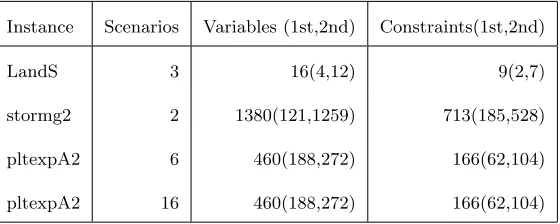
Table 2 and 3 show the characteristics of the original instances and the corresponding inverse problems, respectively.
Table 2: Characteristics of the original instances.
Instance Scenarios Variables (1st,2nd) Constraints(1st,2nd)
LandS 3 16(4,12) 9(2,7)
stormg2 2 1380(121,1259) 713(185,528) pltexpA2 6 460(188,272) 166(62,104) pltexpA2 16 460(188,272) 166(62,104)
Table 3: Characteristics of the inverse instances.
Instance Scenarios Variables (1st,2nd) Constraints(1st,2nd)
LandS 3 103(10,93) 40(4,36)
stormg2 2 6519(427,6092) 2639(121,2518) pltexpA2 6 4326(438,3888) 1820(188,1632) pltexpA2 16 10806(438,10368) 4540(188,4352)
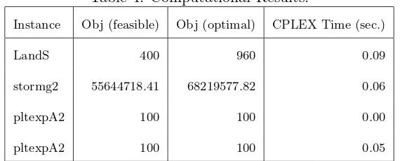
same, q and q′ are the same in some of the instances and q′ < q in others which is an expectable result according to cases established in Section 2.
We leave the exploration of the decomposition algorithms for future work. We anticipate that as the size of the problem increases, decomposition will become essential.
Table 4: Computational Results.
Instance Obj (feasible) Obj (optimal) CPLEX Time (sec.)
LandS 400 960 0.09
stormg2 55644718.41 68219577.82 0.06
pltexpA2 100 100 0.00
pltexpA2 100 100 0.05
Acknowledgments
G. Saka and A. Schaefer were supported by National Science Foundation grants DMI-0217190 and DMI-0355433, as well as a grant from Pennsylvania Infrastructure Technology Alliance. L. Ntaimo was supported by National Science Foundation grant CNS-0540000 from the Dynamic Data Driven Application Systems (DDDAS) Program. The authors would also like to thank Murat Kurt for helpful comments on an earlier version of this paper.
References
[1] R.K. Ahuja and J.B. Orlin. Inverse optimization, Operations Research 49 (2001) 771–783.
[3] E.M.L Beale. On minimizing a convex function subject to linear inequalities, Journal of the Royal Statistical Society, Series B, 17 (1955) 173–184.
[4] J.R. Birge and F. Louveaux, Introduction to Stochastic Programming, Springer, 1997.
[5] D. Burton and Ph.L. Toint. On an instance of the inverse shortest paths problem, Mathematical Programming, 53 (1992) 45–61.
[6] D. Burton and Ph.L. Toint. On the use of an inverse shortest paths algorithm for recovering linearly correlated costs, Mathematical Programming, 63 (1994) 1–22.
[7] S. Coate and B. Knight. Socially optimal districting, NBER Working Paper No. 11462, Available at http://papers.nber.org/papers/w11462.pdf, (2005).
[8] G.B. Dantzig. Linear programming under uncertainty, Management Science, 1 (1955) 197–206.
[9] G.B. Dantzig and P. Wolfe. Decomposition Algorithm for Linear Programs, Econometrica, 29 (1961) 767–778.
[10] J. Day, G.L. Nemhauser and J.S. Sokol. Management of Railroad Impedancies for Shortest Path-based Routing, Electronic Notes in Theoretical Computer Science, 66 (2002) 1–13.
[11] B. Dial. Minimum-revenue congestion pricing, part 1: A fast algorithm for the single origin case, Transportation Research Part B: Methodological, 33 (1999) 189-202.
[12] M.L. Fisher. An applications oriented guide to Lagrangian Relaxation, Interfaces, 15 (1985) 10-21.
[14] D.S. Hochbaum. Inverse problems and efficient convex optimization algorithms. Technical report, University of California, Berkeley, CA., 2004.
[15] ILOG. http://www.ilog.com/.
[16] F.V. Louveaux and Y. Smeers, Optimal investments for electricity generation: A stochastic model and a test-problem, Numerical Techniques for Stochastic Optimization, 445-453. Edited by R. Wets and Y. Ermoliev Springer-Verlag, 1988.
[17] Z. Liu and J. Zhang. Calculating some inverse linear programming problem, Journal of Computational and Applied Mathematics, 72 (1996) 261–273.
[18] R.K. Martin, Large Scale Linear and Integer Optimization: A Unified Approach, Kluwer Academic Publishers, 1999.
[19] J.M. Mulvey and A. Ruszczynski. A New Scenario Decomposition Method for Large-Scale Stochastic Optimization, Operations Research, 43(1995) 477-490.
[20] G. Neumann-Denzau and J. Behrens. Inversion of seismic data using tomographical recon-struction techniques for investigations of laterally inhomogeneous media, Geophysical Journal of Royal Astronomical Society, 79 (1984) 305–315.
[21] G. Nolet. Seismic Tomography, Reidel, 1987.
[22] POSTS. Current List of Available Problems.
http://users.iems.northwestern.edu/ jrbirge/html/dholmes/SPTSlists.html. [23] Slptestset. http://www.uwsp.edu/math/afelt/slptestset/download.html.