University of Karlsruhe (TH) Institute for Economic Policy Research
KEYNEO – a KEYnesian and NEOclassical model of the
German economy
Paper presented to the 23rd International Conference of the System Dynamics Society
July 2005, Boston, USA
Burkhard Schade
University of Karlsruhe
Institute for Economic Policy Research
Institut für Wirtschaftspolitik und Wirtschaftsforschung (IWW) Kollegium am Schloß, Bau IV
76128 Karlsruhe, Germany
Phone: +49 (0) 721 / 608 7690 Fax: +49 (0) 721 / 608 8429 [email protected]
Abstract
The aim of the System Dynamics Model KEYNEO is to model the German economy over a long time period (40 years). Keynesian and neoclassical elements form the base of KEYNEO. In the first step a complex feedback structure was developed to model the main economic variables on an aggregate level. The equations for the supply and the demand side of the economy were defined in the second step.
The results of different runs demonstrate that KEYNEO mimics historic data quite good. With the use of optimization tools the parameters could be estimated. The statistical ana lysis of KEYNEO shows that the results are highly significant. This verification underlines the quality of KEYNEO to model an economy.
1 Introduction
This paper describes the model KEYNEO. The aim of the System Dynamics Model KEYNEO is to model the German economy over a long time period (40 years). This raises the question, which theoretical concepts may serve as base for this system dynamics model. The second chapter discusses evolutionary economics, Keynesian and neoclassical ideas and investigates their potential for a model in system dynamics.
The third chapter describes the system dynamics model KEYNEO itself. Main parts of this chapter are the feedback structure and the explanation of the equations. The fourth chapter analyses the results. It discusses different runs of the model and the parameter estimation.
2 Economic theory and System Dynamics
2.1 Evolutionary Economy and System Dynamics
There seem to be a direct link between evolutionary economy and system dynamics. Evolutionary economy may be described by the following characteristics1:
• path dependency
• multiple equilibrium
• self-organization
• chaotic system behaviour
In system dynamics one may find the same elements. The use of level variables and time variables refers strongly to path dependency. This enables to model irreversible processes and hysteretic.
Equilibrium of level variables may occur when inflow and outflow have the same value. Over time other influences may have an impact on the flow variables and force the system out of the equilibrium. In general, there will be no stable equilibrium over time.
Negative feedback loops stabilize systems. This stabilization might be seen as a characteristic of self-organization process.
Non-linearity’s and the feedback system cause a chaotic behaviour of the system. This may lead to spontaneous reactions and to erratic oscillations2.
The founders of the evolutionary economy didn’t form their ideas in a complete mathematical system. This lead to misperception that evolutionary economics might not be able to develop mathematical models in general. But models from Nelson/Winter and system dynamics models make a contribution to carry out evolutionary ideas with mathematical models3.
2.2 Keynes in System Dynamics
There is strong link between evolutionary economics and Keynesian ideas. Goodwin demonstrates this link4.
Keynes stated that equilibrium only temporarily exists. Markets are too unstable for a general equilibrium. On the goods market there is an ex-ante equilibrium between supply and expected final demand. But ex-post there might be a difference between expected and real
1 See Radzicki, Sterman (1994), S. 64. 2 See Bossel (1994), S. 338ff.
3
See Radzicki (1988), S. 658.
4
final demand. This changes behaviour of economic actors and leads to adaptation processes. These adaptation processes are clearly elements of a self-organized system5.
The behaviour of economic actors depends on previous decisions. This is a characteristic of path dependency. Furthermore, the whole idea of multiplier effects is based on path dependency.
In spite of the rational behaviour of economic actors there might occur a liquidity trap. This liquidity trap can be interpreted as chaotic behaviour.
As there are many similarities between Keynes and evolutionary economics Keynesian ideas are suitable for system dynamics.
2.3 Neoclassic in System Dynamics
Another line of thought that might give some insights to system dynamics is neoclassical ideas. Of course there are in the neoclassical paradigm some assumptions that are contradictory to system dynamics, for instance the equilibrium. Furthermore neoclassical models ignore path dependency and don’t use level variables. However equilibrium conditions might be modeled by negative feedback loops. Therefore neoclassical models can be implemented in system dynamics as complex structures containing only negative feedback loops. The benefit of implanting a neoclassical general equilibrium model in system dynamics is marginal.
It could be worthwhile to implement a neoclassical as a part of a complex system dynamics model. In this case the neoclassical model would form the short-term optimization behaviour of economic actors. The system dynamics model would form the long-term dynamic behaviour of the whole system.
3 The economic Model KEYNEO
The model is based on Keynesian and neoclassical elements. Therefore it is called KEYNEO. The aim of the model is
• to derive a simplified structure of an economy
• to calibrate the model within a long time horizon
• to estimate the parameters
The calibration entails two time horizons. The first time horizon begins in 1960 to 1990, the second in 1991 to 2002. The estimation of the parameters is realized with the optimization tools of Vensim6.
KEYNEO is developed in a way that it is possible to examine separate hypothesis. On the top level the user is enabled to choose between different equations for one variable. For instance, the user has to decide whether the equation for investment consider the nominal interest rate, the real interest rate or no interest rate. Other hypothesis belong to the type of production function, the time delay of the influence of disposable income on consumption and the consideration of business cycles based on the development of the interest rate.
3.1 Qualitative Design of the Model
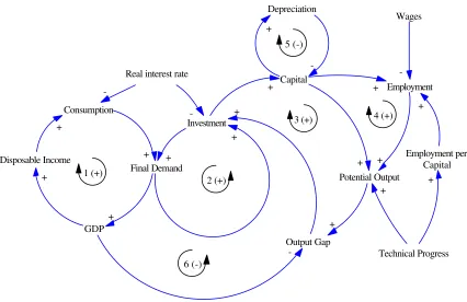
The main feedback loops are designed in the first step. Figure 3-1 shows the main feedback loops.
5
See Goodwin (1991), S. 30.
6
Loop 1 is the consumption feedback loop. Consumption has a positive impact on final demand, final demand on disposable income, and disposable income on consumption. As all impacts are positive this loop is a positive feedback loop.
Loop 2 is the investment feedback loop. Higher investments lead to an increase of final demand and of the expected final demand. Higher expected final demands lead to an increase of investment7. This is also a positive feedback loop.
Loop 3 and 4 relate to the potential output8. The output gap is the difference between the potential output and the gross domestic product (GDP). This output gap has a positive impact on investment. Higher investments lead to an increase of capital. In loop 3 there is a direct link between capital and potential output. In loop 4 a higher capital leads to an increase of employment that increases the potential output.
Figure 3-1: Main Feedback Loops in KEYNEO
Loop 5 is the depreciation loop. Depreciation depends on capital. This feedback loop damps the previous described feedback loops. Loop 6 is also a negative feedback loop. Investment has a positive impact on final demand and GDP. An increase of GDP leads to a decrease of the output gap and this leads to lower investments.
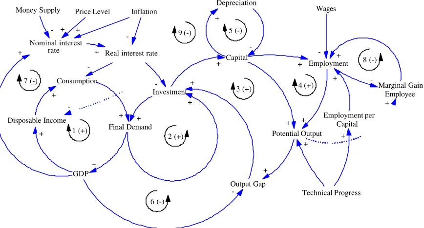
In detail on can find even more feedback loops of KEYNEO (see Figure 3-2). Loop 7 is the interest rate loop. A decrease of the interest rate has a positive impact on investment (and consumption). This leads to an increase of GDP that damps the decrease of the interest rates. Loop 8 balances out the marginal gain of labour with employment. An increase of the marginal gain of labour has a positive impact on employment. The increase of employment leads to a decrease of the marginal gain of labour (by the production function).
7 See Sterman (1986), S. 102. 8
Loop 9 considers that depreciation has to be subtracted from GDP. A decrease of depreciation leads to an increase of GDP and the disposable income. Consumption and final demand will follow this trend. This has a positive impact on investment and capital that increases depreciation. This negative feedback loop is dampened by the effect that an increase of final demand and of GDP leads to an increase of the interest rate (loop 7). This increase damps consumption and investment.
Altogether the model contains four positive and five negative feedback loops. While the four posit ive feedback loops are responsible for the growth of the system, the negative feedback loops stabilize the system.
There are also exogenous factors like money supply, wages and technical progress. Depending on the aim of the modeling this factors should be endogenized.
Disposable Income Figure 3-2: All Feedback Loops in KEYNEO
Figure 3-2 shows that KEYNEO bases more on Keynesian ideas. Investment is calculated with final demand, employment with capital and wages are endogenous.
The use of a production function and of marginal gains relate to neoclassical ideas.
3.2 Development of the System Dynamics Model
3.2.1 Demand side
The main equations on the demand side are defined to calculate consumption and investment. Consumption is derived by the disposable income, a time delay and the interest rate:
C[t]= α·dihh·DI[t-k]β·(1+r)γ (3.1)
with: C: Consumption DI: Disposable Income
dihh: Disposable Income of households to total Disposable Income (Disposable Income HH to Total)
r: Real Interest Rate (Real Interest Rate estimated)
It is assumed that the interest rate has an impact on the evaluation of private assets9. This evaluation has an impact on consumption. Also the German Federal Bank uses interest rates to derive consumption10.
Final demand is the main factor to derive the investments11. Inventory of former period have a negative impact on investment. Interest rates and the output gap play an important role for the calculation of investment:
I[t]= α· (FD[t]-IN[t])·(1-OG)β·(1+r)γ (3.2)
with: I: Investment FD: Final Demand IN: Inventory OG: Output Gap
r: Real Interest Rate (Real Interest Rate estimated) α, β, γ: Parameters
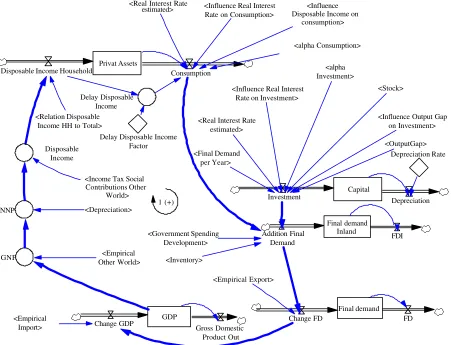
Figure 3-3 describes the demand side in KEYNEO using system dynamics elements. Consumption, investment, government spending and inventory define final demand inland. Exports are taken into consideration to derive final demand. Imports are used to calculate GDP. GDP serves as input to derive gross national product (GNP), net national product (NNP) and disposable income. Disposable income is used to derive private assets and consumption.
Privat Assets
Disposable Income Household Consumption
<Relation Disposable Income HH to Total>
<alpha Consumption>
Figure 3-3: Demand side (Feedback Loop 1) in KEYNEO
9 See Sargent (1994), S. 47f. 10
See Deutsche Bundesbank (1996), S. 32. This impact is hard to verify empirically.
11
3.2.2 Supply side
Main variables on the supply side are capital, employment and potential output. Capital can be derived by investment minus depreciation. It is assumed that value of depreciation depends more on depreciation rules. For this reason one can assume a fix depreciation rate on capital.
K[t+1]=K[t] + (I[t] – K[t]·dpr)·dt (3.3)
with: K: Capital I: Investment
dpr: Depreciation Rate dt: time step
Employment is derived within several steps. In the first step the employment is calculated based on information about the current situation. The second step takes into consideration that employment markets react sluggish. They adapt at the current situation with a certain time delay.
In general, it is assumed that employment depends mainly on investment and capital12. Therefore the relation between employment and capital multiplies capital. Furthermore, the relation between marginal gain of labour and wages are taken into consideration. Wages are not derived by the assumption of equilibrium. They depend on the specific current situation in the society13.
with: ELT: Employment long term K: Capital Stock
empc: Employment per Capital
mge: Marginal Gain per Employee per Month W: Empirical Wages Per Employee
α, β: Parameters
Employment per capital is modeled as a level variable with the unit person per million DM14. Each period employment per capital is decreasing by a certain factor. This factor depends on technical progress. It is also considered that the decrease is lower when employment per capital is already low.
empc[t+1] = empc[t] - α·(empc[t])β·tp·dt (3.5)
with: empc: Employment per Capital tp: Technical Progress
dt: time step α, β: Parameters
The marginal gain of labour is calculated from the derivative of the function of the potential output:
with: mge: Marginal Gain per Employee per Month PP: Potential output
E: Employment
β: Elasticity of labour in the production function
It is assumed that employment markets react sluggish. The calculation of the current employment considers the employment of the former period and the long term employment:
12 See Keynes (1973), S. 98f. 13 See Keynes (1973), S. 5ff. 14
E[t+1]=E[t] + α·(ELT[t] – E[t])·dt (3.7)
with: E: Employment
ELT: Employment long term α: Parameter
The production function is a Cobb-Douglas-Function. Employment and capital serve as main input. Technic al progress is treated as exogenous:
[ ]
= ⋅ λ⋅ ⋅[ ] [ ]
α⋅ β t E t K e c tPP t (3.8)
with: PP: Potential Output K: Capital Stock E: Employment c: Const GDP
λ: rate of technical progress (Lambda GDP) α: elasticity of capital (Alpha GDP) β: elasticity of Labour (Beta GDP)
To derive the potential output full employment and full use to capacity is not considered. In this model potential output is calibrated with GDP.
3.2.3 Link between Demand and Supply
The difference between GDP and potential output is the output gap15 (see Figure 3-4).
t €
GDP Potential output
Output gap
Figure 3-4: GDP, Potential Output and Output Gap
The output gap is derived as follows:
OG = (PP – GDP)/PP (3.9)
with: OG: Output Gap PP: Potential Output GDP: GDP
The output gap has an important influence on the investment (see equation 3.2). If the potential output is above GDP than there is a positive impact on investment. If it is below GDP than there is a negative effect on investment. This link combines the supply side with the demand side.
15
3.2.4 Money
The interest rate can be calculated by money supply and money demand. It follows from this that an increase of GDP and of the price level has a positive impact on nominal interest rates. Money supply has a negative influence on the interest rate16. In the model the real interest rate is derived endogenous while the inflation is exogenous.
(
)
(1 i)with: nr: nominal interest rate (Nominal Interest Rate estimated) GDP: GDP
M3: Money supply M3 (Emirical M3) PN: Price level (Empirical Price Level) i: Inflation (Empirical Inflation) α,β,γ,δ: Parameters
Real interest rate can be calculated with the nominal interest rate minus inflation:
r = nr - i (3.11)
with: r: Real Interest Rate (Real Interest Rate estimated)
nr: Nominal Interest Rate (Nominal Interest Rate estimated) i: Inflation (Empirical Inflation)
The real interest rate has an impact on consumption and investment (see equation 3.1 and 3.2).
3.2.5 Variants
During the model development several hypothesis have been verified. One variant from the basic model is the consideration of a specific business cycle. These business cycles depend on expectations of economic actors. It was assumed that economic actors consider the development of the final demand and the interest rates in the past for their current decisions. For the final demand this assumption could not be confirmed, but for the interest rates. This means that economic actors assume a continuation of the trend of the interest rate. If there is a break in the trend then the reactions of actors are higher than in the normal case (no break). The trend of the interest rates is derived by the average interest rate of a number of years:
∑
with: r: average real interest rate (Interest expected) r: Real Interest Rate (Real Interest Rate estimated) k: Number of Years
The current trend of the interest rate is derived by the difference between the current interest rate and the average interest rate.
α
with: tr: difference to trend of interest rates (Trend Difference Interest Rate) r: average interest rate (Interest expected)
r: current interest rate (Real Interest Rate estimated) α: Parameter
If this current trend of the interest rate is considered in the equation of the employment then one can reach better results for the development of employment.
16
4 Results of the Model
Two runs were made with KEYNEO. Run 1 covers the time period from 1960 to 1990, run 2 from 1991 to 2002. Figure 4-1 shows the results of these runs in one diagram.
Consumption : Run 1960 - 2002
Investment : Run 1960 - 2002
Final demand : Run 1960 - 2002
4000
1960 1971 1982 1992 2003
6
Empirical Consumption : Run 1960 - 2002 2 2 2 2 2
3 3 3 3 3
Empirical Investment : Run 1960 - 2002 4 4 4 4
5 5 5 5 5
Empirical Final Demand : Run 1960 - 2002 6 6 6 6
Figure 4-1: Results of Consumption, Investment and Final Demand
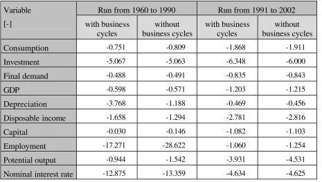
Consumption, investment and final demand of the model show a high correspondence with their empirical developments. The derivation between calculated and empirical data is derived using the optimization tools of Vensim17. The results are described in Table 4-1.
Table 4-1: Results of the calibration of KEYNEO
Run from 1960 to 1990 Run from 1991 to 2002
Nominal interest rate -12.875 -13.359 -4.634 -4.625
17
For all variables the derivation is below 31 respectively 12. This means that the model meets empirical data under a significance of 95%.
The variant with the business cycles has mainly better results for the employment.
In the whole, the most problematic variables are employment, investment and interest rates. These variables are very volatile and therefore it is more difficult to derive the exact developments of them.
In spite of this volatility Figure 4-2 shows that employment figures of KEYNEO meet the empirical development quite good.
40
1960 1971 1982 1992 2003
2 2
Figure 4-2: Results for employment
We can see the same for the interest rates. The peaks in the year 1973 and 1980 can be derived with the model.
12
1960 1971 1982 1992 2003
2
2
2 2
1 1
1
Real Interest Rate estimated : Run 1960 - 2002 1 1 1 1
Empirical Interest Rate : Run 1960 - 2002 2 2 2 2
1 1
2 2 2
year
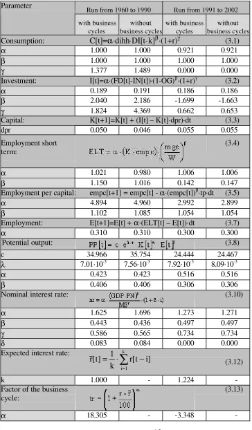
For both runs we use the same structure but different parameter estimation. Table 4-2 shows the result of the parameter estimation for the two runs.
For the investment multiplier the results are quite similar. In all cases the investment multiplier is around 0.19 of the final demand. The influence of the interest rate is a bit lower for the run 2 (1991-2002). The depreciation rate is around 5% for all runs.
Table 4-2: Results of the parameter estimation in KEYNEO
Run from 1960 to 1990 Run from 1991 to 2002
Potential output: (3.8)
c 34.966 35.754 24.444 24.467
λ 7.01·10-3 7.56·10-3 7.92·10-3 8.09·10-3
α 0.423 0.423 0.516 0.516
β 0.406 0.406 0.306 0.306
Nominal interest rate: (3.10)
α 1.625 1.696 1.273 1.271
β 0.443 0.436 0.497 0.497
γ 0.586 0.565 0.734 0.734
δ 0.083 0.084 0.000 0.000
Expected interest rate:
Concerning the trend of the employment per capital the model derives a lower decrease for run 2 than for run 1. A reason of this effect could be that other market effects dampen the influence of technical progress.
The elasticity’s of capital are higher than the elasticity’s for labour in all runs. The gap between the elasticity’s increases in run 2. This means that in the current time the factor capital is even more important than in former times. The parameter technical progress is very narrow in all runs.
It is remarkable that the parameter of the output gap changes the sign. This parameter links the demand and supply together. A possible interpretation for this effect is the following. During the time between 1960 and 1990 the production function and the potential output is the dominating element. If it is higher than GDP then there is an increase of investment. After 1991 the demand is the dominating element. If GDP is higher than potential output then there is an increase of investment.
The results for the parameters of the interest rate are also very close together in all runs. Only the parameter for the inflation has in run 2 no impact. A reason may be that after 1991 the inflation was very low and stable.
5 Conclusion
Besides evolutionary economics the model bases on a combination of Keynesian and neoclassical elements. Of course some of the elements have to be modified to fit with the system dynamics philosophy. In some cases the level- variable concept and time delays have to be added.
Altogether the results demonstrate that the model generates the development of the main variables of the German economy. The calibration and the statistical analysis show a high correspondence to real data. The calibration of employment, interest rate and investment is most difficult. The development of interest rates may depend on variables out of the system boundaries, e.g. currencies. With respect to employment information about part time, protection against dismissal and governmental debts are not considered. However, the results of the statistical analysis are for all variables within the 95% interval and therefore highly significant. This verification underlines the quality of KEYNEO to model an economy.
In addition, the structure of KEYNEO may serve as input for much more sophisticated models like ESCOT (model for Economic assessment of Sustainability poliCies Of Transport)18.
6 Appendix
Bossel, H. (1994): Model building and simulation (Modellbildung und Simulation). Vieweg, Braunschweig/Wiesbaden.
Deutsche Bundesbank (1996): Econometric Multi-Country-Model (Makro-ökonometrisches Mehr-Länder-Modell). Deutsche Bundesbank, Frankfurt.
Goodwin, R. M. (1991): Schumpeter, Keynes and theory of economic evolution. Evolutionary Economics, Vol. 1, Issue 1, pp. 29-47.
18
Keynes, J. M. (1973): The general Theory of employment interest and money. University Press Cambridge, Cambridge.
Läufer, N. K. A. (1994): Money Supply (Geldangebot). B. Mohr (Paul Siebeck), Tübingen. Peterson, D. W. (1980): Statistical Tools for System Dynamics. In: Randers, J. (Hrsg.):
Elements of the System Dynamics Method. Productivity Press, Cambridge.
Radzicki, J. M. (1988): Institutional Dynamics: An Extension of the Institutionalist Approach to Socioeconomic Analysis. Journal of economic issues, Vol. 22, Issue 3, p633, 33p. Radzicki, M.; Sterman, J.D. (1994): Evolutionary Economics and Systems Dynamics. In:
England, R.: Evolutionary Concepts in Contemporary Economics, University of Michigan Press, Michigan.
Radzicki, J. M. (2004): Ecpectation Formation and Parameter Estimation in Uncertain Dynamical Systems: The System dynamics Approach to Post Keynesian-Institutional Economics. Paper for the twenty-second conference of the System Dynamics Society, Oxford.
Sargent, T. (1994): Macro Economics (Makroökonomik). Verlag Oldenbourg, München/Wien.
Schade, B.; Rothengatter, W. (2004): The Economic Impact of Environmentally Sustainable Transport in Germany. Journal of European Transport and Infrastructure Research, Vol. 4, No. 1, pp. 147-172.
Schade, B.; Rothengatter, W.; Schade W. (2002): Strategies, Policies and Economic
Assessment of Sustainable Transportation with the System Dynamics Model ESCOT (Strategien, Maßnahme n und ökonomische Bewertung einer dauerhaft
umweltgerechten Verkehrsentwicklung. Bewertung der dauerhaft umweltgerechten Verkehrsentwicklung mit dem systemdynamischen Modell ESCOT (Economic assessment od Susainability poliCies Of Transport)). Erich Schmidt, Berlin. Schweppe, F. C. (1973): Uncertain dynamic systems. Prentice-Hall, Englewood Cliffs. Sterman, J. D: (1986): The economic long wave: theory and evidence. System Dynamics
Review, Vol. 2, No.2, pp. 87-125.