English translation © 2012 M.E. Sharpe, Inc., from the Russian text © 2011 “Ekonomika i biznes.” “Makroekonomicheskaia model’ laffero-keinsianskogo sinteza,” Ekonomika i biznes, 2011, no. 3 (May–June), pp. 11–34. A publication of the Faculty of Economics and Business, Ivane Javakhishvili Tbilisi State University.
Iuri Ananiashvili is a Doctor of Economic Sciences and a professor in the Department of Econometrics, Ivane Javakhishvili Tbilisi State University; e-mail: iuri_ananiashvili@ yahoo.com. Vladimer Papava is a Doctor of Economic Sciences, professor, corresponding member of the National Academy of Sciences of Georgia, and chief research fellow at the Paata Gugushvili Institute of Economics; e-mail [email protected].
Translated by James E. Walker.
© 2012 M.E. Sharpe, Inc. All rights reserved. ISSN 1061–1991/2012 $9.50 + 0.00. DOI 10.2753/PET1061-1991541202
I
URIA
NANIASHVILIANDV
LADIMERP
APAVAMacroeconomic Model of
Laffer-Keynesian Synthesis
The article presents a macroeconomic equilibrium model in which aggregate demand and aggregate supply are considered not in relation to the price level, as is traditionally done, but in terms of functions dependent on the average tax rate. The concepts of optimal and equilibrium tax rates are introduced. In the former case, aggregate supply is maximum, while in the latter case aggregate demand and supply coincide. Based on an analysis of the model, it is shown that when the government tries to maintain the equilibrium average tax rate at a fixed level, the optimal tax rate becomes dependent on the price level, and an appropriate change in aggregate demand may lead to approximation of the optimal rate to the equilibrium rate. It is also demonstrated that each given value of the equilibrium tax rate can be matched with a set of functions and curves of aggregate supply and the national budget’s tax revenues.
economics, in which the effect of the tax rate on aggregate supply is brought to the fore. The role of taxes can be fully explained, and the one-sided nature of these two theories can be overcome through a synthesis of supply-side economics and Keynesianism, which was first suggested by one of the present authors.1
The model presented below is a further development of this idea of a Laffer-Keynesian synthesis. It is based on a macroeconomic equilibrium model that con-sists of aggregate demand and aggregate supply functions. However, in contrast to the standard models of aggregate demand and aggregate supply, these functions are analyzed not in the coordinates of a plane on the axes of which values of the price level P and output Y are shown, but on a plane in which the vertical axis corresponds to the average tax rate t; and the horizontal axis, to output Y. In this model, the price level, together with the rest of the factors that affect aggregate demand and aggregate supply, is exogenously given.
Model of aggregate demand
We begin our analysis with an examination of aggregate demand functions, which we designate as YD(t). This notation indicates that aggregate demand YD is considered in the form of functions of the average tax rate t. Based on a modified version of a simplified Keynesian model, it has been shown2 that, if analysis is limited just
to the product market, then the aggregate demand function that depends on the average tax rate can be expressed in the following form:
Y t A
t b tg D
( )
( ) ,
=
− − −
�
1 1
(1)
where A} is planned autonomous spending; this parameter is the sum of autonomous household consumption a, autonomous government purchases G}0,3 gross domestic
private investments I0, and net exports NX0:
A} = a + G}0 + I0 + NX0;
b is the marginal propensity of households to consume, 0 < b < 1; and g is the marginal propensity for government purchases, 0 ≤g ≤ 1.
To give the aggregate demand function its final form, it is advisable to expand our analysis and, along with the product market, also look at the money market. For this purpose, we represent gross domestic investments I0, which are a part of autonomous spending, not in the form of an exogenous quantity, but in the form of a function that depends on the interest rate:4
I0 = I0 – µi,
to the interest rate; i is the nominal interest rate. The value of i is established in the money market by the mechanism of balancing the money supply and demand. In the simplest case, the equation corresponding to equilibrium of the money market can be represented in the following form:5
M
P kY t hi
D
= ( )− ,
where M/P is the real cash balance of money in circulation (it is determined by the ratio of the nominal amount of money M and the price level P); and k, h are posi-tive coefficients expressing the sensitivity of the demand for money to aggregate spending YD(t) and the interest rate i.
Taking the equations given above into account in (1) and making the appropriate transformations, we get the following model of aggregate demand:6
Y t A
Here the quantity A consists of exogenously given elements. In particular,
A a G I NX
NX0, A also contains an element that is determined by the real cash balance of money (M/P).
It can be shown7 that the properties of function (2) are determined by the
inter-relation of the marginal propensity to consume b and the marginal propensity for government purchases g. All else being equal, YD(t), in the area of its determination,8
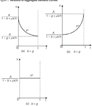
is increasing in relation to t when g > b, decreasing when g < b, and indifferent when g = b.9 A graphic illustration of the function YD(t) with various possible combinations of values of b and g is given in Figure 1. It should be noted that, all else being equal, a change in A, which is determined from (3), shifts the curves corresponding to YD(t). In particular, with an increase in A, the curves YD(t) shift upward in parallel, which for a given average tax rate means an increase in ag-gregate demand. On the other hand, with a decrease in A the curves YD(t) shift downward in parallel, which for a given average tax rate corresponds to a reduction in aggregate demand.
Model of aggregate supply
As the aggregate supply that depends on the average tax rate we can consider a function of total output that fully satisfies the conditions of the Laffer theory and has the following form:10
YS(t) = Y
where Y
pot expresses the volume of potential output with full use of economic resources in conditions of the existing technology; f(t) = –etδlntδ is a function that reflects the institutional aspect and determines the cumulative tax effect on sup-ply. This is a behavioral function; it shows the degree of use of existing economic resources with a given value of the average tax rate (i.e., in conditions of a given institutional environment). Based on this content, f(t) should satisfy the condition 0 ≤f(t) ≤ 1. When f(t) takes a value close to 1, this indicates that economic activ-ity is high for the given average tax rate and the level of use of resources is close to the maximum. The opposite situation takes place when f(t) is close to zero. In this function, e represents the base of the natural logarithm, and δ is a positive parameter that we will discuss later.
Figure 1. Versions of Aggregate Demand Curves
(b) (a)
(c)
b > g b < g
0
YD
0 0
1 t
b = g
1 t
YD
Y
YD
Y
A A
A A
1 t
1 – b + µk/h
1 – b + µk/h A
Y
1 – b + µk/h 1 – g + µk/h
We have investigated the properties of the aggregate supply function (4)11 and
of resources, and output is maximum, that is, it is at the potential level Ypot. Con-sequently, t* can be considered the optimal average tax rate.
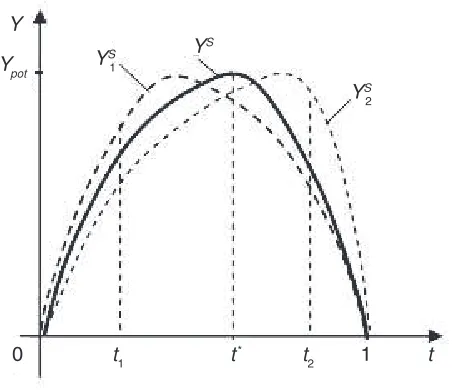
A graphic illustration of function (4) is given in Figure 2 (the curve YS). It shows that when all else is equal, movement on the ascending part of the curve corresponds to a change in the average tax rate from 0 to t*; and movement on the descending
part of the curve YS, to a change from t* to 1.12
What happens if “all else being equal” changes?
First we should point out that in the conditions of model (4) for aggregate supply, a change in all else being equal involves a change either in the amount of potential output (Ypot) or in the value of parameter δ. As a rule, a change in Ypot occurs mostly in the long term, and the reason for such a change may be an increase or decrease in labor or the existing amount of capital, improvement or deterioration in the quality of technologies, a change in labor productivity, and so on. When these changes have a positive effect on Ypot, then the curve YS(t) shifts upward on the coordinate plane (aggregate supply increases, i.e., with the existing average tax rate more products and services will be produced in the economy than there were before the increase in Ypot). Obviously, a decrease in the amount of potential output will cause the opposite result: the curve YS(t) will shift downward and, in conditions of the existing tax rate, aggregate supply will decrease. Interestingly, when all else being equal is unchanged, neither an increase nor a decrease in potential output affects the optimal value of average tax rate t*. In other words, with a change in Ypot, the maximum of function (4) changes, but the value of the tax rate at which this maximum is attained does not change.
A completely different situation occurs when a disruption of all else being equal in the aggregate supply model (4) involves a change in the current market condi-tions, price level, production costs per unit of output, or producers’ expectations. These circumstances, especially a change in the price level, do not have affect the amount of potential output Ypot or, accordingly the maximum value of the function
YS(t); however, they do affect parameter δ and the optimal tax rate determined by this parameter.13 In other words, for example, with an increase in the price level
the maximum value of the function YS(t) will not change; however, the value of the average tax rate at which this maximum is attained will change.14 Consequently,
in this case, a graph of the function YS(t) will shift (deviate) from the position YS to the right or left. In Figure 2, the dashed curves Y1S and Y
2
of the shift (deviation). The specific direction of the shift (deviation) depends on which of the intervals [0, t*) or (t*, 1] the existing tax rate is in. If we assume that
the current rate is in the interval [0, t*) and, for example, is t
1 (t1∈ [0, t *), then
with an increase in the price level, the graph of the function YS(t) will shift to the position Y1S, while if we take t
2 as the existing rate, which is in the interval (t *, 1],
that is, t2∈ (t*, 1], then the shift (deviation) will be to the right, to the position Y2S.15 The standard premise known from economics courses—that if there is not
full employment, an increase in the price level (or a decrease in production costs per unit of production, or improvement of the current market conditions, etc.) has a positive effect on aggregate supply and causes it to increase—is fulfilled in the process of these changes.
Macroeconomic equilibrium model
Using the aggregate demand models (2)–(3) given above and the aggregate supply model (4), we will write the condition of macroeconomic equilibrium YS(t) = YD(t), determined in relation to the average tax rate, as follows:
Y et t A
t b tg k h pot( ln )
( ) / .
− =
− − − + δ δ
µ
1 1 (5)
Equation (5) is a condition of Laffer-Keynesian equilibrium. It shows that for macroeconomic equilibrium to exist, all else being equal (for the given values of autonomous spending, the real cash balance of money, and potential output), the tax Figure 2. Aggregate Supply Curve and Versions of Its Movement
Y
Ypot
0 t1 t* t
2 1 t
YS
1
YS
YS
rate t must be such that it satisfies equation (5). We will call this t the equilibrium average tax rate.16 The existence of equilibrium t is graphically illustrated in Figure 3,
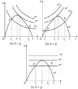
where YS represents the aggregate supply curve; and YD, the aggregate demand curve. In this case, Figure 3a corresponds to the case when in YD(t) the marginal propensity for government purchases g is less than the marginal propensity to consume b; Figure 3b, to the case when g > b; and Figure 3c, to the case when g = b.17
As we see, with different relationships of b and g for given values of autono-mous spending A}0, the real cash balance (M/P), and potential output Ypot, three cases can take place:
1. No equilibrium average tax rate exists (the curves YS and YD do not intersect). It is clear that this happens when autonomous spending A}0, which is part of A, is so large that potential output Ypot is not enough to satisfy it.
2. There are two equilibrium values of the average tax rate, t1 and t2 (the curves YS and YD intersect at two points), the role and values of which are determined by Figure 3. Equilibrium in Conditions of Laffer-Keynesian Synthesis
Y Y
Y
YD
YD
YD
YD
YD
YD
YD
YD
YD
0 t1 t* t
2 1 t
0 t1 t* t′
1 t2 1 t 0 t1 t′1 t
* t
2 1 t
(a) b > g (b) b < g
(c) b = g F
F
F E
E
E
YS
the relationship between the marginal propensity of households to consume b
and the marginal propensity for government purchases g. When b > g (Figure 3a), of the two equilibrium values of the average tax rate the lower one t1 is preferable, since it provides for greater aggregate spending; for the same reason, in the case of b < g (Figure 3b), the higher tax rate t2 is preferable; and finally in the case of b = g (Figure 3c), both rates t1 and t2 provide the same result from the point of view of production, employment, and aggregate spending. 3. There is a single equilibrium tax rate (curves YS and YD touch each other at only
one point). In the case of Figures 3a and 3b, this rate cannot be optimal. Henceforth, for the sake of simplicity, of the three different relationships of b and
g we will consider only one. In particular, we will assume that b > g. We pointed out above that in this situation aggregate demand YD(t) is a decreasing function in relation to the average tax rate and this fully conforms to Keynesian theory. Here we note that the results for the case considered here are the same as those obtained in the other two cases.
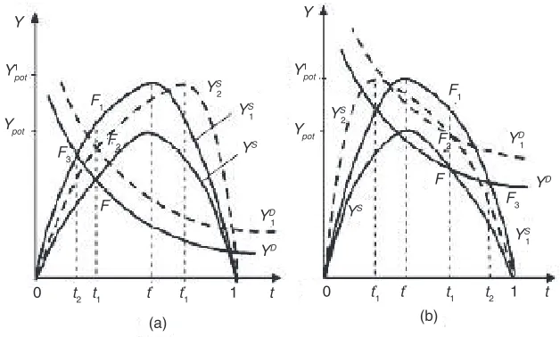
Versions of disruption and restoration of equilibrium
To clarify how equilibrium is established in conditions of the given model, we turn to equation (5). Since for this equation the cases of nonexistence of a solution or the existence of only one solution (the first and third of the cases indicated above) are highly unlikely, we will assume that, for the given values of A, Ypot, and δ, in relation to t (5) has two solutions: t1 and t2. Consequently, for curves YS and YD given in Figure 4, macroeconomic equilibrium can be found at one of the points F
and E. For clarity, we will assume that the starting point of economic equilibrium is F, which corresponds to the average tax rate t1.
Suppose that, for certain reasons, the initial equilibrium is disrupted. As follows from (5), the reason for this could be:
• achangeinaggregatedemandduetoanumberofcircumstances,includingan
increase or decrease in one or more of the elements of planned autonomous spending or the real cash balance;
• apurposefulchangeinthetaxratebythegovernment;
• achangeinaggregatesupplyduetoanincreaseordecreaseinpotentialoutputYpot. We will consider each case separately.
Restoration of equilibrium in the case of a change in aggregate demand
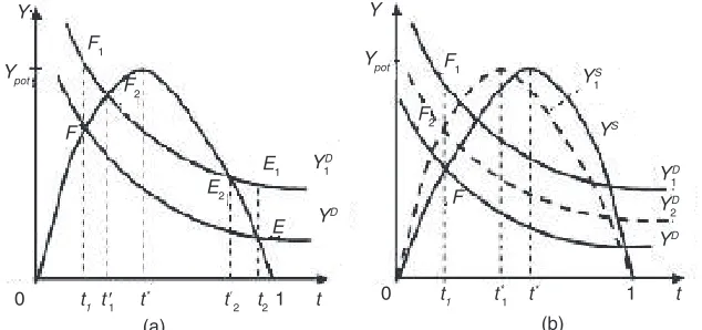
a shift of the aggregate demand curve YD to a new position Y
1
D (see Figure 4a). In the new situation that is created, as long as the tax rate is at level t1, the amount of increased aggregate demand is determined by point F1 and is greater than the amount of aggregate supply, which, for its part, is determined by point F. Depend-ing on what actions the government takes, restoration of equilibrium or transition to a new equilibrium can be accomplished in two ways.
One way to establish equilibrium is to step up government activity, in par-ticular, for it to improve tax administration and, by applying appropriate laws, to increase the value of t from t1 to t1′, in parallel with the growth of autonomous spending. Such a measure will have an effect on the amount of aggregate demand as well as aggregate supply: increasing the tax rate will reduce the amount of aggregate demand (on the aggregate demand curve Y1D it moves from point F
1 to F2) and, according to the Laffer theory, increase the amount of aggregate sup-ply (on the aggregate supsup-ply curve YS it moves from point F to F
2). As a result
of these changes, a new equilibrium corresponding to the increased output is established at point F2.
If the initial point of the economy’s equilibrium was not at point F, but at E, the situation would be different. According to Figure 4a, the latter point (i.e., E) is on the descending part of the aggregate supply curve, where the negative effects of taxes play a dominant role. Therefore, if in the hypothetically created situation the government lowers the value of t from t2 to t′2, then the economy will be able to make the transition to a new equilibrium E2 and ensure that the increased aggregate demand is properly satisfied.
from regulating the tax rate, then other mechanisms go to work, one of the most important of which is the market mechanism of regulation by prices.
From the standard model of aggregate demand and aggregate supply, which is analyzed in coordinates of the plane of price level and total output, it follows that when the economy is in a state of less than full employment and excess demand occurs,18 then, all else being equal, the price level rises. In the general case, this
causes a decrease in aggregate demand and an increase in aggregate supply, so that equilibrium is established between them. Naturally, this mechanism also oper-ates, with a certain specific nature, in the model (2)–(5) that we are examining. Its specific nature in model (2)–(5) is that in conditions of a fixed average tax rate an increase in the price level has an effect on the location of the aggregate demand and aggregate supply curves and causes them to shift.19 The form and direction of this
movement for the case when the initial macroeconomic equilibrium is at point F
are shown in Figure 4b. Here, curves YD and Y
1
D express aggregate demand before the rise of the price level. In this case, YD is the initial curve, and Y
1
D is the curve that occurred after the increase in autonomous spending. Curve YS corresponds to the supply that existed before the change in the price level.
The aggregate demand curve, which was lowered as a result of the rise of the price level,20 will take position Y
2
D, and the curve for the increased aggregate supply will take position Y1S
. Consequently, the new equilibrium established as a result of
the change in the price level is determined by point F2.
We point out the circumstance that, in conditions of a fixed tax rate, a change in the price level caused by a change in autonomous spending and, accordingly, aggregate demand, has an effect on parameter δ and on the optimal tax rate deter-mined by this parameter. When the initial equilibrium point is on the ascending part of aggregate supply (as it is in the case considered above), that is, when the tax rate t1 corresponding to equilibrium is less than its optimal value t*, the growth
of aggregate demand and the price level are accompanied by a process of decrease of parameter δ and movement of the optimal tax rate to the left. In this case, if the process of growth of aggregate demand continues and, consequently, the price level also continues to rise, a time will come when the optimal tax rate becomes equal to the given fixed value of t1 corresponding to equilibrium.
The opposite situation takes place when the initial equilibrium point is on the descending part of curve YS and the tax rate corresponding to equilibrium is greater than its optimal value t*. In these conditions, with a fixed value of the tax
rate, growth of aggregate demand and, accordingly, the price level causes growth in parameter δ, a shift of the aggregate supply curve to the left, and movement of the optimal tax rate toward the rate corresponding to equilibrium. In this case, if aggregate demand increases to a certain level, then the tax rate corresponding to the initial equilibrium will become the optimal rate.
Restoration of equilibrium in the case of a change in the tax rate
We consider the case when the reason for disruption of equilibrium F is a purpose-ful change in the tax rate t1 by the government. As in the previous case, we will assume that the average tax rate t1 (see Figure 5a), which is less than the fiscal Laffer point of the first kind t*,21 corresponds to the initial equilibrium. Suppose
that the government has decided to switch to optimal taxation t* and has raised the
average tax rate accordingly. All else being equal, according to the Laffer theory, because of the dominance of positive effects, transition to the new tax regime t*
will cause a growth in aggregate supply, which will be reflected accordingly on curve YS: there will be a transition from point F to point F
2. At the same time, the
increased tax rate will have an effect on aggregate demand, and movement from point F to point F1 will begin on curve YD. Consequently, as we can see from Figure 5a, an increase in the tax rate in some period will lead to the appearance of excess supply. In the situation that has been created, there are two possible ways of restoring equilibrium.
In one of them, in parallel with increased taxes, the government should promote growth of aggregate demand, for example, by making additional autonomous purchases or conducting an expansionary monetary policy. This will be a logical continuation of the actions that it has begun. If the government can increase the aggregate A (which consists of elements of autonomous spending and the real cash balance) to the level22A = Y
pot[(1 – b) + t*(b – g) + µk/h] in this way and the aggregate demand curve is shifted to position Y1D, then equilibrium is restored, with output reaching its potential value, so that the price level will not change (Figure 5a).
From the version of establishing equilibrium considered here, it follows that just putting the optimal tax rate into effect cannot ensure employment growth and initiate Figure 5. Restoration of Equilibrium in the Case of a Change in the Tax Rate
the transition to equilibrium corresponding to potential output. In conditions of a Laffer-Keynesian synthesis, along with the tax regime, aggregate demand plays a significant role in achieving increased economic activity and full employment.
And the second way of restoring equilibrium convinces us of this. In fact, sup-pose that the government has limited itself to just increasing the tax rate and does not take any additional measures to stimulate aggregate demand. Then the task of overcoming the imbalance that has been created is shouldered by the economy’s main market mechanism; the price regulation mechanism. The point is that excess aggregate supply stimulates a reduction in the price level. In this process, aggregate demand begins to grow, and its curve shifts upward, from position YD to position
Y1D, while aggregate supply decreases, and its curve shifts from position YS to the right, to position Y1S (Figure 5b).23 Ultimately, a new equilibrium will appear
at point F2 instead of F, and it will correspond to less than the potential output. Moreover, rate t* will lose the function of optimality, and in the situation that has
been created the role of the optimal tax rate will be assigned to t1*. Consequently,
the government’s attempt to create full employment in the economy exclusively by adjusting the tax rate will not be successful if it is not assisted by appropriate aggregate demand.
Restoration of equilibrium in the case of a change in aggregate supply
Another cause of disruption of equilibrium could be a change in factors deter-mining the level of potential output, for example, an increase or decrease in the existing amount of labor or capital, or deterioration or improvement in the level of technology. In all of these cases, Ypot, which is part of the aggregate supply function, undergoes a change and, because of this, aggregate supply also changes. Geometrically, this circumstance is expressed in a shift of aggregate supply curve
YS, except that, in contrast to the movements considered previously, in this case YS shifts upward if Ypot increases, and downward if Ypot decreases.
Suppose that, in conditions of initial equilibrium F, the value of potential output was Ypot, and the aggregate supply corresponding to it was described by curve YS (Figure 6). Say that the value of Ypot has increased to Y1
pot because of an improvement in technology. All else being equal, this will cause a shift of the aggregate supply curve to position Y1S and a temporary disruption of equilibrium: for the existing tax rate t1, output will reach point F1, provided that aggregate demand is determined by point F. A situation of excess aggregate supply is created, and there are three ways to bring it back into equilibrium:
equilibrium output in Figure 6a and lower equilibrium output in Figure 6b. 2. In conditions of the existing tax rate, by means of fiscal and monetary policy,
the government should encourage an increase in aggregate demand to a level such that curve YD shifts to point F
1. If this happens, then the new equilibrium
will be at point F1.24
3. If the government does not intervene in the process of creating equilibrium, then, because of the excess demand, the mechanism of self-regulation will take effect, and the price level will decline. On the one hand, this will increase aggregate demand, and the aggregate demand curve will shift to position Y1D; on the other hand, it will decrease aggregate supply and shift the aggregate supply curve from position Y1S to Y
2
S. In the end, a new equilibrium position will be created at point F2, at which the level of output and employment are higher than at the initial equilibrium point F.
We will call attention to the circumstance that, even in this case, a change in the price level causes a shift of the aggregate supply curve, and this is once again followed by a change in the optimal tax rate, which shifts from point t* to t
1 *.
Hence the conclusion can be drawn that when the government keeps the average tax rate in a stable position, then each new equilibrium price level has its own optimal tax rate.
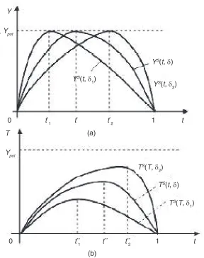
The Laffer curve
Analysis of model (2)–(5) of Laffer-Keynesian equilibrium has shown that when the tax rate is fixed, changes that occur in the economy have an effect on the aggregate Figure 6. Effect of a Change in Potential Output on the Equilibrium Position
supply function (4) and cause a change in parameter δ. This means that each given value of the equilibrium tax rate can correspond to a whole set of aggregate supply functions and, accordingly, supply curves that differ from each other in the value of parameter δ (or in the value of the optimal tax rate t*, which is the same thing).
Because of this, aggregate supply YS can be seen as a function of two variables,
t and δ:
YS = YS(t, δ).
In this notation, all else being equal, t reflects the weight of the tax burden. As for δ, to explain its content we have to take into account the circumstance that the aggregate supply model (4) is, in essence, a behavioral model expressing the result of economic agents’ expected response in conditions of a tax burden of one weight or another. Naturally, in various situations existing in the economy, this response may not be the same for the same tax burden, the more so as the behavior and de-cision making of most economic agents is based on rationalism. And the latter, as we know, implies that economic agents optimize their behavior not just once, but over and over, continuously, taking each new circumstance into account. Conse-quently, parameter δ quantitatively expresses the result of the circumstances that may have an effect on the nature of the relationship that exists between aggregate supply and the tax burden.25
Like the aggregate supply function, the version of the budget revenues function
TS(t) determined on the basis of the supply function, that is, the Laffer function, should be seen as a function of two variables. In the conditions of model (2)–(5) under consideration here, it has the following form:
TS (t) = tYS(t) = Y
It can be shown that tax rate t** corresponding to the maximum of the Laffer
function (6), which is also called the Laffer point of the second kind,26 is
deter-mined as follows:27
and, like the supply curves, a set, or family, of Laffer curves is obtained.28 However,
in contrast to the aggregate supply curve, which has the same value of the maximum
Ypot for all δ, the maximum value of the Laffer curve (6) is different for various δ. The point is that for function (6), the following condition takes place:29
Therefore, with a change in δ, the value of the tax rate t** corresponding to the
maximum of the Laffer curve changes, as does the maximum amount of tax revenues
TS(t**, δ) that can be obtained with that tax rate. In particular, TS(t**, δ) increases
with an increase in δ and decreases with a decrease. Consequently, a shift of t** to
the right on the tax rate axis is accompanied by an increase in TS(t**, δ).
Figure 7 shows aggregate supply curves and the budget revenues correspond-ing to them for different values of δ. In both parts of the figure (7a and 7b), it is understood that the relationship δ1< δ < δ2 takes place.
Figure 7. Set of Aggregate Supply and Laffer Curves
Y
Ypot
YS(t, δ
1)
YS(t, δ)
YS(t, δ
2)
0 t*
1 t
* t*
2 1 t
(a) T
Ypot
TS(T, δ
2)
TS(t, δ)
TS(T, δ
1)
0 t**
1 t
** t**
2 1 t
Suppose that, in a state of macroeconomic equilibrium, the aggregate supply curve corresponding to the given rate t is YS(t, δ), and the Laffer curve is TS(t, δ) (see Figure 7). Say that, in these conditions, aggregate demand has increased, and the government has decided to keep the tax rate at the existing level t. We already know that when the initial macroeconomic equilibrium is on the ascending part of the supply curve YS(t, δ), then in the newly created situation, new aggregate supply
YS(t, δ
1) and Laffer functions and curves T
S(t, δ
1) will be formed, and the δ1
cor-responding to these curves is less thanδ2. If we assume that, in the same situation, the initial macroeconomic equilibrium is on the descending part of the supply curve
YS(t, δ), then the new aggregate supply and Laffer functions and curves take the form determined by YS(t, δ
2) and T
S(t, δ
2), respectively. It is clear that opposite changes
will occur in the case of a decrease in aggregate demand: the aggregate supply and Laffer curves will shift to positions YS(t, δ
2) and T
S(t, δ
2), respectively, if the initial
macroeconomic equilibrium is on the ascending part of the initial equilibrium, and to the positions YS(t, δ
1) and T
S(t, δ
1), if it is on the descending part.
From the analysis that has been done, it follows that the Laffer curve is not a stable construct and can change depending on the situation that has been created in the economy, especially as a result of a change in the price level, which also implies a change in t**. In such conditions, the widespread opinion among
pro-ponents of the theory that it is desirable to somehow determine the value of the tax rate t** that provides maximum tax revenues to the budget, which is the basis
for developing economic policy and improving the existing tax regime, loses its attractiveness, since, because of the changes occurring in the economy, it will be necessary to change the established rate and in the final analysis this will produce an undesirable result.30
Notes
1. V. Papava, “The Georgian Economy: from ‘Shock Therapy’ to ‘Social Promotion,’”
Communist Economies and Economic Transformation, 1996, vol. 8, no. 2.
2. Iu.Sh. Ananiashvili and V.G. Papava, “Rol’ srednei nalogovoi stavki v keinsianskoi modeli sovokupnogo sprosa,” Obshchestvo i ekonomika, 2010, no. 3–4.
3. To be more precise, G}0 includes not the full amount of government purchases (as is customary in traditional Keynesian models, but only the part of it that does not depend on tax revenues to the national budget and is determined exogenously.
4. See, for example, R. Dornbush [Dornbusch] and S. Fisher [Fischer], Makroekonomika
[Macroeconomics] (Moscow: MGU INFRA-M, 1997), p. 117. 5. Ibid., p. 131.
6. It should be noted that (2) differs from the well-known version of the Keynesian model of aggregate demand (from the IS–LM model) in the rule that reflects taxes and determines the aggregate A of autonomous elements.
7. Ananiashvili and Papava, “Rol’ srednei nalogovoi stavki v keinsianskoi modeli sovokupnogo sprosa.”
9. A detailed explanation of the reasons why aggregate demand is increasing in relation to the tax rate when b < g is given in Ananiashvili and Papava, “Rol’ srednei nalogovoi stavki v keinsianskoi modeli sovokupnogo sprosa.”
10. Iu. Ananiashvili, “Vlianie nalogov na sovokupnoe predlozhenie,” Ekonomika da biznesi, 2009, no. 1 (in Georgian).
11. Iu. Ananiashvili and V.G. Papava, “Modeli otsenki vlianiia nalogov na rezul’taty ekonomicheskoi deiatel’nosti,” Ekonomika, Finansy, Nalogi, 2010, no. 2.
12. It is assumed that an increase in the tax rate is accompanied by positive and negative effects. For a value of the average tax rate in the range from 0 to t*, the sum of the positive effects exceeds the sum of the negative ones, and therefore movement on the ascending part of the aggregate supply curve corresponds to an increase in the tax rate in this interval. The opposite relationship of positive and negative effects occurs for subsequent values of the average tax rate, and so a decrease in aggregate supply corresponds to an increase in the tax rate in the section (t*, 1] . For a detailed explanation of this question, see ibid.
13. Recall that in the aggregate supply model (4), t* and parameter δ are interrelated as
t* = e–1/δ.
14. The case when the economy is in a state of full employment and tax rate t coincides with optimal value t* is an exception. In this case, an increase in the level of prices does not affect either the maximum of the function YS(t), the parameter δ, or the tax rate t* correspond-ing to it. Consequently, in this case the aggregate supply curve stays where it is.
15. It is easy to notice that when the aggregate supply curve shifts to the right, the value of the optimal tax rate decreases, and when the curve shifts to the left, it increases. Taking this into account, from the expression determining the optimal tax rate (t* = e–1/δ), we will establish that a decrease in the value of parameter δ corresponds to a shift of the curve YS(t) to the left; and an increase in δ, to a shift to the right.
16. Based on the specifics of equation (5), in the general case it is not possible to derive an analytical expression for equilibrium t, but it is no problem to find it by approximate calculation methods.
17. Recall that in the suggested version of the Keynesian model of aggregate demand, the relationship of the b and g determines the nature of the dependence of aggregate demand on the average tax rate. In particular, YD(t) decreases in relation to t when b > g, increases when b < g, and is indifferent when b = g.
18. We are dealing with precisely such a case.
19. A change in the price level within the limits of model (2)–(5) means a disruption of “all else being equal.” Therefore, on the coordinate plane of the tax rate and output a change in the price level has an effect on the location of the curves YD and YS, while in the standard model of aggregate demand and aggregate supply, a change in the price level causes move-ment on the curves YD and YS.
20. The point is that when P rises, all else being equal, A decreases, since the latter includes the element M/P, which depends on P (see equation [3]).
21. E.V. Balatskii [Balatsky], “Analiz vliianiia nalogovoi nagruzki na ekonomicheskii rost s pomoshch’iu proizvodstvenno-institutsional’nykh funktsii,” Problemy prognoziro-vaniia, 2003, no. 2.
22. This formula is directly derived from (5) by substituting t* into it and taking into account that f(t*) = –e(t*)δln(t*)δ = 1.
23. We pointed out above that in model (2)–(5) a change in the price level affects the position of the aggregate demand and aggregate supply curves.
25. As we pointed out above, among these circumstances a special role is played by a change in the price level, therefore, instead of δ we can use the notation δ = δ (P), and the notation of the aggregate supply function YS(t) can be replaced by YS = YS(t, δ(P)).
26. E.V. Balatskii [Balatsky], “Effektivnost’ fiskal’noi politiki gosudarstva,” Problemy prognozirovaniia, 2000, no. 5.
27. Ananiashvili and Papava, “Modeli otsenki vlianiia nalogov na rezul’taty ekono-micheskoi deiatel’nosti.”
28. It should be noted that there are now many articles and studies confirming or refuting the concept of the Laffer curve and problems of its practical realization (see, e.g., V. Papava, “Lafferov effect s posledeistviem,” Mirovaia ekonomika i mezhdunarodnye otnosheniia,
2001, no. 7; V. Papava, “On the Laffer Effect in Post-Communist Economies (On the Basis of the Observation of Russian Literature), Problems of Economic Transition, 2002, vol. 45, no. 7, pp. 63–81). Some of them deny the existence of this curve, and some confirm it a priori. But, except for the case of dividing the curves into long- and short-term periods (Dzh.M. B’iukenen [J.M. Buchanan] and D.R. Li [Lee], “Politika, vremia i krivaia Laffera” [Politics, Time, and the Laffer Curve], in M.K. Bunkina and A.M. Semenov, Ekonomicheskii chelovek: V pomoshch’ izuchaiushchim ekonomiki, psikhologiiu, menedzhment (Moscow: Delo, 2000), all of them unequivocally analyze a single curve, rather than a set of curves.
29. Ananiashvili and Papava, “Modeli otsenki vlianiia nalogov na rezul’taty ekonomi-cheskoi deiatel’nosti.”
30. In the opinion of the well-known economist Robert Barro, constant changes in the tax rate (either increases or decreases) cause greater distortions and irrecoverable losses than a tax regime that has a fixed rate (see, e.g., Dzh. Saks [J. Sachs] and F.B. Larren [Lar-rain], Makroekonomika. Global’nyi podkhod [Macroeconomics in the Global Economy] [Moscow: Delo, 1996], p. 245).