129
5
Consumer Theory
C O N C E P T S
● Total Willingness to Pay ● Consumer Surplus
● Cash Subsidy ● Kind Subsidy
● Direct Tax ● Indirect Tax
C
onsumer theory has numerous applications. In this chapter we consider four of them. The first one is an application of the marginal utility theory, while the remaining three are applications of the indifference curve analysis.CONSUMER’S SURPLUS
We have learnt that if the price of a product falls (or rises), all else the same, the consumer is always better off (or worse off). It is useful to express such ‘welfare’ change in terms of money (or rupees). Why? Suppose that the government slashes the duty on printers imported from abroad. Obviously, those who purchase print-ers are better off. We would like to know how much money or purchasing power they gain, because of this policy change, in terms of their command to buy goods and services in general. As another example, suppose that the government increases the entertainment tax on movies and, as a result, the movie tickets become costlier by 20 per cent. Those of you who are avid movie goers would not like it. It is a loss of purchasing power to you. One may want to know how much purchasing power the movie goers are losing because of this tax policy change.
There are a few measures that quantify the welfare change in terms of money due to a price change. Of these, the most commonly used is called the consumer surplus, defined as the total willingness to pay for a product minus the total pay-ment for the product.
If we are talking about good x, for example, and pxand xstand respectively for the price and the quantity demanded of this good, the total payment for good xis simply price ×quantity demanded =pxx.
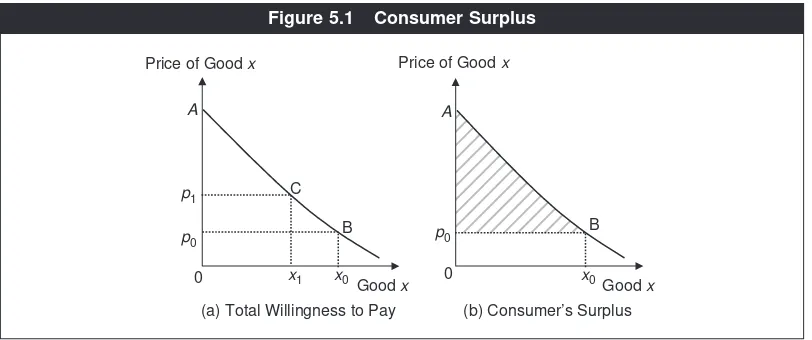
The total willingness to pay for good xis defined as the total utility obtained from consuming x, measured in terms of money. It is the maximum amount that the consumer is willing to pay for the product. From the marginal utility theory, remember that this is measured by the area under the marginal utility (in terms of money). Further, this curve is same as the demand curve for the product. Hence the total willingness to pay is equal to the area under the demand curve. Turning to Figure 5.1(a), if px=p0and the consumer is demanding x0, her total willingness to pay is equal to the area 0ABx0. Similarly, if px=p1and the consumer demands x1, the total willingness to pay equals the area 0ACx1.
We are now ready to compute consumer surplus. If the price is p0, for instance, the total willingness to pay =0ABx0, while the total payment is equal to the area 0p0×0x0=0p0Bx0. Thus the consumer surplus=0ABx0− 0p0Bx0=p0AB. By similar calculation, at the price p1, the consumer surplus is equal to p1AC. In general, we then say that the consumer surplus equals the area under a demand curve over and above the line representing the price. For example, in panel (b) of Figure 4.23, the shaded area shows the consumer surplus at the pricep0.
The negative sign reflects a welfare loss due to a price increase, which is expected. In absolute value, the change in the consumer surplus equals the area between the two respective price lines.
See Clip 5.1 for a sample of estimates of consumer surplus. A
(b) Consumer’s Surplus B p0
x0Good x 0
C A
(a) Total Willingness to Pay x1
B p1
p0
x0
Price of Good x
Good x 0
Price of Good x
Figure 5.1 Consumer Surplus
Clip 5.1: Consumer Surplus Estimates
Many estimates of consumer surplus are available for various commodities and services in India and other countries. For instance, Watal (2000) provides estimates of loss in consumer surplus in the demand for patentable pharma-ceutical products if intellectual right protections are granted in India following our WTO commitments. Assuming that prices of such products would increase anywhere from 26 per cent to 242 per cent, the consumer surplus loss is evalu-ated at 50 million to 140 million US dollars. Peck, Chaloupka, Jha and Lightwood (1999) study the demand for tobacco products in India and China (and in other countries). They estimate that, in per capita terms and on 1990 prices, the consumer surpluses in demanding tobacco products are 12 US dol-lars and 9 US doldol-lars in India and China respectively. Mitra (1999–2000) has examined the demand for four tourist spots in Arunachal Pradesh. Using local transport cost as the price of touring these spots, the consumer surplus per visit by Indians is estimated at Rs 995; that by foreigners is estimated at Rs 1, 232.
References
Mitra, Amitava. 2000. Environmental Conservation and Demand for Nature-Based Tourism in Arunachal Pradesh: Final Report. Submitted to Environmental Economics Research Committee, IGIDR, funded by World Bank Aided: Environmental Management Capacity Building Technical Assistance Project.
NUMERICAL EXAMPLE 5.1
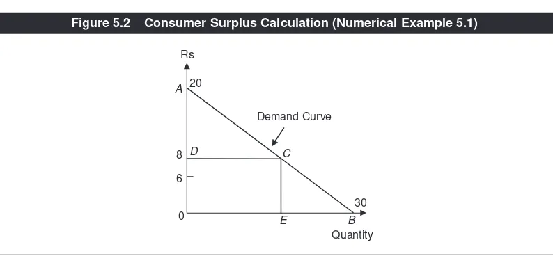
The demand curve facing a consumer is a straight line as shown in Figure 5.2. What is the consumer’s total willingness to pay for the product if the price is equal to 8? Derive the consumer surplus at price equal to 6 and price equal to 8. Compare the two surpluses. Which one is greater and why?
At price = 8, we have AD=20 −8 =12. The triangles ADCand A0Bare similar.
Thus DC/AD= 0B/0A. The last ratio equals 30/20 = 3/2. Thus DC= (3/2)AD = (3/2)12 = 18. This is the quantity demanded at price equal to 8. The total willing-ness to pay at this price is equal to the area under the demand curve, which, in turn, equals the areas of rectangle 0DCEplus the triangle ADC. These areas are respectively equal to 8 ×18 = 144 and (1/2) ×12 ×18 = 108. Thus the total
will-ingness to pay = 144 + 90 = 234. The consumer surplus is the area of the triangle under the demand curve, equal to 108.
Similar calculation yields the consumer surplus at price 6 equal to 147. This is higher than the consumer surplus at price equal to 8, because the price is lower.
CASH VERSUS KIND SUBSIDY
The government offers many types of ‘kind subsidy’ to poor sections of the popu-lation or to its employees. For instance, food in the canteens of many government organisations is highly subsidised. A decent meal with 3 chapatis, dal, asubji and
0 8
30 6
20 Rs
Quantity Demand Curve
B C
E D
A
Figure 5.2 Consumer Surplus Calculation (Numerical Example 5.1)
Peck, Richard, Frank J. Chaloupka, Prabhat Jha and James Lightwood. 1999. ‘A Welfare Analysis of Tobacco Use,’ in Prabhat Jha and Frank J. Chaloupka (eds), Curbing the Epidemic: Governments and the Economics of Tobacco Control. Washington D. C.: World Bank.
curd may cost an employee Rs 5, whereas the market price of that meal is Rs 20. Another example is LTC (leave travel concession) given to central and state gov-ernment employees. This is again a subsidy in kind; the govgov-ernment is subsidising its employees’ ‘consumption’ of travel.1
Note that, in each of these examples and in general, providing subsidy in kind costs something to the government (and ultimately to tax-payers). The objective behind providing a kind subsidy is to improve the welfare of the recipients.
There is, however, an alternative, which will cost the same to the government and also please its recipients—that is, let the government pay cash to the recipi-ents (called a cash subsidy) equal to the amount it was spending on the subsidy programme in kind. The issue is—which programme is better for the consumer given that both programmes cost the same to the government?
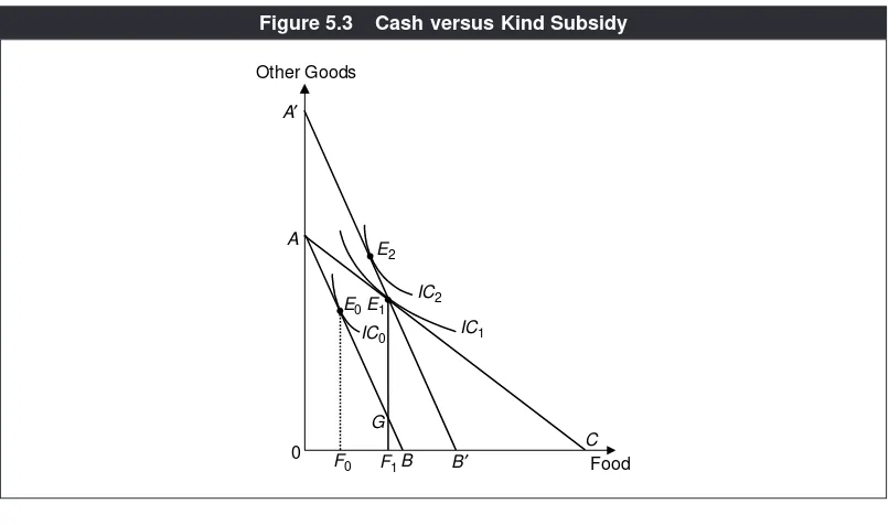
We analyse this by referring to Figure 5.3. It measures food on one axis and ‘other goods’ (by virtue of the composite-good theorem) along the other. Suppose that without any subsidy on food, the budget line of the consumer is AB.
The slope of ABmeasures the relative price of food. The consumer attains his
equilibrium at E
0. He consumes F0of food and E0F0of other goods. His welfare is
indicated by the indifference curve IC
0.
Suppose the government subsidises the consumption of food (that is, food becomes cheaper to the consumer) such that the new budget line is AC. The person
would now consume F
1of food and E1F1of other goods. Mark the point G, where
E
1F1 intersects AB. We can now argue that E1G is the cost of this kind-subsidy
IC1 IC2 E1 IC0 E2 A
B
C Food Other Goods
B′ F1 A′
E0
G
0 F
0
Figure 5.3 Cash versus Kind Subsidy
1In the US, the poor are given ‘food stamps’ by the government, which can be used as cash only if the person is buying
programme. How? Suppose the consumer was buying the same amount of food he is consuming now (F
1) at the unsubsidised (old) price, that is, along the old budget line AB. He would then have been left with GF
1of other goods. But with the sub-sidy programme in place, he is left with E
1F1of other goods. Since the prices of other goods are unchanged, the difference between E
1F1and GF1, equal to E1G, must be what the government is paying as the subsidy.
Consider now the alternative programme of giving the amount E
1Gby cash to the consumer. Mark the line A’B’drawn parallel to ABand passing through E
1. It has the property that E
1G =AA’. With the cash subsidy in place, in terms of the other goods the consumer’s disposable income (inclusive of the cash subsidy) is now 0A+E
1G= 0A+AA’ =0A’. Since there is no subsidy on food, the new budget line must have the original slope AB. Thus A’B’ is the budget line. What is then the consumer’s optimal point of consumption? It is E
2. Note that the optimal con-sumption point in the subsidy-in-kind programme, which is E
1, is still available to the consumer in the cash-subsidy programme (as E
1lies on A’B’ too). But, E1is no longer the equilibrium point. Importantly, at E
2the consumer is on a higher indif-ference curve (IC
2) as compared to that at E1 (IC1).
The conclusion is that the consumer is better off in the cash-subsidy programme than in the kind-subsidy programme. The underlying economic reason is the following. The cost of the kind-subsidy programme (E
1G) depends on the equi-librium choice of the consumption bundle in that programme; hence in a cash-subsidy programme whose cost is equal to the kind-cash-subsidy programme, the above consumption bundle is also available (that is, the bundle E
1 is available along the budget line A’B’). This implies that the consumer cannot be worse off in the cash-subsidy programme as compared to the kind-subsidy programme because he always has the option of choosing E
1in the cash-subsidy programme. Moreover, since the relative price of the good in question facing the consumer is different between the two schemes, he will choose a different bundle in the cash-subsidy programme (E
2) than the one in the kind-subsidy programme (E1) and be better off in choosing so. Put differently, moving from the kind-subsidy pro-gramme to the cash-subsidy propro-gramme provides ‘trading opportunities’ to the consumer in terms of choosing his consumption bundle. This opportunity to trade enhances his utility.2
Our conclusion then raises a question, that is, why do we observe kind-subsidy in practice? One explanation is that the consumer, in accordance with his own preferences, may spend the cash-subsidy on items that the government does not want him to spend on, for example, alcohol. Many poor people, especially men, are indeed addicted to drinking and if any extra cash is given to them, intended to be spent on food, it is likely to be spent instead on alcohol. Our indifference curve model and our conclusion that a cash-subsidy programme is better than a kind-subsidy programme implicitly assume that the pattern of preferences of the targeted recipients is not ‘perverted’ from the viewpoint of the government.
2To carry forward the argument, the equilibrium bundle in the cash-subsidy programme is not available in the kind-subsidy
DIRECT VERSUS INDIRECT TAX
Taxes are of two kinds. One is a direct tax, referring to a tax on an individual or
an organisation. Direct taxes include personal income tax, corporate income tax, wealth tax, property tax and gift tax. In India, only the central government imposes personal income tax. There are no state income taxes. In some countries like the US, some states also levy income tax over and above the central (federal) income tax. Corporate income tax is levied on the profits of private companies. After this tax is paid, a company may invest a part of the remaining profits in building assets for the company or it is paid out to shareholders as dividends. Dividend income, as wage income, is subject to personal income tax. Direct taxes are those that cannot be shifted to other parties.
The other is an indirect tax, referring to taxes, which alterthe cost or price of a
good or service for either producers or consumers. There are many types of indi-rect taxes used in India (and other countries), such as import or customs tariff, excise tax, sales tax, service tax and value added tax (VAT).
Suppose the government wants to generate a given amount of revenue from consumers or households for spending on national defence, building a dam, sub-sidies for the poor and so on. There are two options: an income tax as a direct tax and an indirect tax on a commodity or service. Which is the better option for the sake of consumer’s welfare?
In many ways this issue is analogous to the earlier one of kind versus cash sub-sidy, which involved the method of disbursing among a class of people a given amount of tax revenue already raised rather than raising revenue itself. Note that an indirect tax increases the price of a product for the consumer and hence is the opposite of a kind subsidy. Further, an income tax is the opposite of a cash sub-sidy. But, interestingly, the answer to both the issues is similar. Income tax is a better option in terms of consumer’s welfare, just as cash subsidy was shown to be better for the consumer than kind-subsidy.
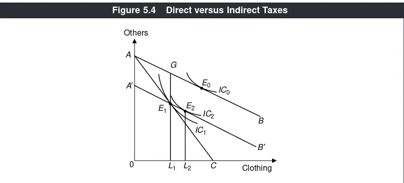
Turn to Figure 5.4. There are two goods: clothing and ‘others’. Suppose there is no tax to begin with. The price line is AB. The consumer’s equilibrium is at E
0.
First consider a sales tax on clothing. The price of clothing is higher for the con-sumer because of this tax. Let ACbe the new price line. The consumer chooses the
tangency point E
1. She consumes L1of clothing and E1L1of ‘others’. The
indiffer-ence curve passing through E
1is at a lower level than the one passing through E
0—as you would expect, the consumer is worse off than before. How much
rev-enue is the government collecting? The answer is GE
1. It is because if the
con-sumer did not have to pay the sales tax, she would have had GL
1 of ‘others’ but
she actually has E
1L1of ‘others’. Therefore, the difference, equal to GE1, must be
the sales tax proceeds.
If, instead of the sales tax, the amount GE
1is taken away from the consumer
as income tax, her budget line is A’B’, parallel to AB. The point E
2is the
equilib-rium point. Notice that the consumer is on a higher indifference curve (IC 2) in
The economic reason behind this is similar to that in the case of kind versus cash subsidy. In the income tax programme, the equilibrium bundle with the indi-rect tax programme (E
1) is available to the consumer. Thus the consumer cannot be worse off than in the indirect tax programme. The relative price of clothing is different between the two programmes. Hence, in the income tax programme, the consumer will pick a bundle (E
2) other than (E1) and be strictly better off com-pared to the indirect tax programme.
Why do governments then use indirect taxes? The prime reason is that an income tax is politically unattractive in the sense that it is visible and affects an individual’s pocket directly. On the other hand, the cost of an indirect tax is less visible to the public and hence politically more convenient. Moreover, the author-ity to impose a direct tax like an income tax lies with the central government only, not with state governments. Hence, state governments, in order to raise revenues for their expenditure and commitments, resort to indirect taxes.
CONSUMPTION-SAVINGS DECISIONS
The last chapter dealt with the consumer’s decision-making on how much to con-sume of different goods and services. More generally, we can think of the follow-ing decision problems facfollow-ing an individual or a family. After it receives its income, a part of it is spent and the remainder is saved. How much to spend and how much to save is one problem. The second problem is to allocate the total spending on different goods and services (which we studied in the last chapter).3
E0
L2 E2 A
B
C Others
Clothing A′
B′
E1 G
0 L1
IC0
IC1 IC2
Figure 5.4 Direct versus Indirect Taxes
Interestingly, the method we undertook to analyse the second problem can be applied to understand the first problem. This is the objective here: to analyse a consumer’s decision with regard to consumption and savings.
Recall the composite-good theorem which says that if the relative prices among any bunch of goods remain unchanged, the total spending on these goods can be interpreted as a single good. Assuming that the relative prices among all goods the consumer buys do remain constant, we can them lump the total spending on them as one good, say ‘consumption’ or ‘present consumption’. Now realise that people save so that they can use their savings towards consumption in the future. In other words, we can say that a consumer uses his income to meet present con-sumption as well as future concon-sumption.
Assume for simplicity that a consumer lives only two periods, present (period 1) and future (period 2), that is, there is only one future period. This will imply that such a consumer will only save in period 1 to be used for consumption in period 2. (As the world ends after period 2, so to speak, there is no point in sav-ing anythsav-ing in the terminal period 2.)
In this scenario we can now frame the choice problem of a consumer in a pre-cise way. Let C
1, Sand Y1denote a person’s consumption, savings and income in period 1. By definition, S =Y
1 −C1. Note that savings can be positive, zero or neg-ative. Negative savings mean that C
1 > Y1, that is, the excess of consumption over income is financed by borrowing. Similarly, positive savings mean lending. If you keep your savings in a bank, it is like lending your savings to the bank. Let r
denote the market interest rate at which one can borrow or lend. If a person saves amount S
0, the principal plus interest to be received or paid in period 2 is equal to
S
0(1 + r), depending on whether S0is positive or negative.
Budget Line
Let C
2and Y2denote consumption and income in period 2. What is the relation-ship between C
This is the intertemporal budget equation facing the individual.4The left-hand
side is the discounted value of present and future consumptions, whereas the right-hand side is the discounted value of present and future incomes. The word ‘discounted’ means that future consumption and future income are adjusted to make them comparable to present consumption and present income. For instance, while C2is the future (period 2) consumption it is worth only C2/(1 +r) in terms of the period 1. That is, if you forgo C2/(1 + r) amount of consumption today (period 1) and save, it will fetch you (1 +r)[C2/(1 + r)] = C2of consumption in period 2.
We assume that the present and future incomes are given to the consumer.5In
this scenario, the consumer faces a choice problem involving C1 and C2. Indeed, you can think of C1and C2like two goods in the last chapter. In view of the budget equation (5.1), the price of present consumption is p1 =1 and the price of future
con-sumption is p2 =1/(1 +r).
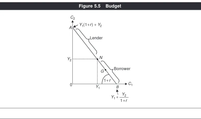
Figure 5.5 depicts the budget line AB. If C2=0, then C1=Y1+Y2/(1+r). Thus
Y1 + Y2/(1 + r) is the intercept of the budget line on the x-axis measuring C1. Likewise, you can determine that the intercept on the y-axis measuring C2is equal to Y1(1 +r) +Y2. The absolute value of the slope of ABis then:
4The word ‘intertemporal’ means ‘over time.’
5For example, Y
1can be your present salary in period 1 and Y2your expected salary in period 2. Or if you own some rental
The term 1 +ris indeed the relative price of present consumption in terms of
the future consumption, as p1/p2=1/[1/(1 +r)] = 1 +r. This has a straightforward
interpretation—if the interest rate is r, as you sacrifice one unit of present con-sumption (that is, save one unit), you get future concon-sumption equal to 1 + r.
There is a particular point on ABwhich is of special significance. Look at the point N, where C1= Y1and C2= Y2, that is, the present consumption is exactly
equal to the present income and future consumption matches with future income. This is the point at which there is no borrowing or lending, that is, savings are zero. If the consumer chooses a point on ABand below the point N, like G, then
C1>Y1. This means that he is a borrower. Similarly if he chooses a point on AB
lying above the point N, then he is a lender.
However, before looking at which point the consumer will choose (in princi-ple), let us consider how the budget line shifts when the current income (Y1) future income (Y2) or the interest rate (r) changes. Suppose Y1increases. Then the inter-cept on the x-axis moves to the right and that on the y-axis moves up. Thus the budget line shifts to the right. The same holds for an increase in Y2. But an increase in the interest rate has a different kind of effect. Note three things. (i) A higher
rmeans a lower value of Y1+Y2/(1 +r), implying that the intercept on the x-axis
shifts towards the origin. (ii) This means a higher value of Y1(1 +r) +Y2and thus
the vertical intercept moves up. (iii) Think about the point N—since it is the zero borrowing-lending point, it must remain unaffected by any interest rate change. Put differently, the choice of C1=Y1and C2=Y2always satisfies the budget
irre-spective of what the interest rate is. That is, the point Ndoes not move. These three features imply that the budget line shifts neither to the right nor to the left entirely. Instead, an interest rate increase moves the budget line clockwise, pivot-ing on the pointN. This is shown in Figure 5.6.
0 C2
C1 N
B A
Preferences and Consumer’s Equilibrium
Which point on the budget line will be chosen by the consumer? It would partly depend on the preferences about present and future consumption. All else the same, if he is very impatient he would have a lot of present consumption and a lit-tle of future consumption. If he is very patient, he would choose the opposite. Indeed, C
1 and C2, can be thought of as two goods (like ice-cream and chocolate). Accordingly, we can draw indifference curves for C
1and C2, and define the mar-ginal rate of substitution of present consumption for future consumption as the units of future consumption the consumer wants to forego in order to have one extra unit of present consumption. This is called the intertemporal rate of substi-tution.Denote this as MRS
12. Recall that, in general, MRS is equal to the slope of the indifference curve. Hence MRS
12is equal to the slope of the IC in present and future consumption.
Once all this is understood we can readily characterise the consumer’s equilib-rium. Turn to Figure 5.7. Given his budget, the consumer maximises his utility from present and future consumption at the point of tangency between the budget line and the indifference curve. In panel (a) this is indicated at the point E
G.
Panel (b) represents a different individual with a generally flatter indifference curve with the equilibrium point being E
H. In both cases, the tangency point
between the indifference curve and the budget line is the equilibrium point. What is the general condition of consumer’s equilibrium? The tangency point has the property that the slope of the IC = the slope of the budget line. Or
MRS
12=1 +r.
There is, however, an important qualitative difference between the two panels. In panel (a), the consumer is a borrower (as E
savings are negative. In panel (b), the consumer saves a positive amount and is a lender (as EHlies above Non the line AB).
Realise now that what we have outlined so far is an economic analysis of con-sumption and savings as an application of the indifference curve analysis. We can now further apply it to understand how income and interest changes affect these decisions.
Changes in Incomes and the Interest Rate
Suppose there is an increase in the present income. This shifts out the budget line and the situation is exactly analogous to income effect studied in the last chapter. It is reasonable to assume that both current consumption and future consumption are normal goods (since these are broad aggregates rather than specific goods). This means that as the present income increases, current consumption and future consumption both increase. What about savings? Since future consumption also increases with present income, only a fraction of an increase in present income goes towards present consumption. This implies that savings increase.
In macroeconomics you must have come across the concepts marginal
propen-sity to consume (MPC) and marginal propensity to save (MPS). In the present context they are defined respectively as the increase in present consumption and
savings per unit increase in present income. What we are saying then is that MPC
>0 and MPS>0. Further, both MPCand MPSbeing positive, and because MPC+
MPS= 1, it follows that 0 <MPC, MPS<1.
We thus have a ‘microeconomic foundation’ here as to why MPC and MPS are positive and less than one. The important underlying assumption is that both cur-rent consumption and future consumption are normal goods.
Consider now an increase in future income. This also shifts out the budget line and given our assumption of ‘normality’, it means an increase in present and future consumption also. However, as the present consumption increases while the present income is unchanged, it implies a decrease in the savings.
Since the budget line shifts out in each case, the consumer is always on a higher indifference curve. That is, a consumer always benefits from an increase in the present income or the future income.
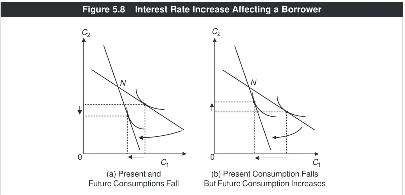
This result can be explained in terms of substitution and income effects. An increase in the interest rate increases the relative price of present consumption in terms of future consumption (that is, present consumption is now more ‘expen-sive’ relative to future consumption than before). Thus, by the substitution effect, the consumer will reduce current consumption and increase future consumption. Furthermore, since he is a borrower, an increase in the interest rate reduces his real income. Assuming normality, this would tend to reduce both present and future consumptions. Hence the net effect is that present consumption decreases unam-biguously whereas future consumption may increase or decrease.
How does an increase in the interest rate affect savings? Mark that present con-sumption falls, while there is no change in the present income. This implies that savings, equal to the excess of present income over present consumption, increase.6
Does the consumer benefit or lose, in terms of welfare? See that in both panels the consumer moves to a lower indifference curve. Thus he is worse off. Why? Because he is a borrower, an increase in the interest rate tends to reduce his real income.
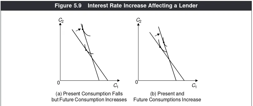
The lender’s case is shown in Figure 5.9. Combining the effects shown in both panels we see that as the interest rate rises, present consumption may increase or decrease while future consumption increases unambiguously. It is because, by the substitution effect, present consumption falls and future consumption rises as in the case of a borrower. But, being a lender an increase in the interest rate tends to increase real income. Given normality, this would tend to increase consumption in both periods. Therefore, the net effect on present consumption is ambiguous, while that on the future consumption is positive.
How are savings affected? Since present consumption may increase or decrease while the present income remains the same, unlike for the borrower, the lender’s
0
N
C1 C1
C2 C2
(a) Present and Future Consumptions Fall
(b) Present Consumption Falls But Future Consumption Increases
N
0
Figure 5.8 Interest Rate Increase Affecting a Borrower
savings may increase or decrease. The reason lies in the underlying substitution and income effects. Finally, we notice from Figure 5.8 that a lender is always better off with a higher interest rate. This is expected, since an increase in the interest rate tends to increase the real income of a lender.
C1 C1
C2
0 C2
0
(b) Present and Future Consumptions Increase (a) Present Consumption Falls
but Future Consumption Increases
Figure 5.9 Interest Rate Increase Affecting a Lender
Economic Facts and Insights
● Consumer surplus measures the level of welfare associated with a
particu-lar price of a commodity.
● An increase (or a decrease) in the price of a product leads to a decrease
(or an increase) in the consumer surplus.
● Equilibrium consumption bundle in a kind-subsidy programme is always
available in a cash-subsidy programme but not vice versa (presuming that both programmes involve the same amount of subsidy). Thus the latter pro-gramme offers more trading opportunities compared to the former and hence is preferred by the consumer.
● Equilibrium consumption bundle in an indirect tax programme is always
available in an income tax programme but not vice versa (presuming that both programmes yield the same amount of revenues). Thus the latter pro-gramme offers more trading opportunities compared to the former and hence is preferred by the consumer.
● A person’s savings can be interpreted as his future consumption.
● The interest rate reflects the relative price of present consumption in terms
of future consumption.
E
E X
X E
E R
R C
C II S
S E
E S
S
5.1 What is the definition of consumer surplus?
5.2 Your house-maid asks you for her Diwaligift. You offer her either Rs 100 or
some item of Rs 100 that she can use. Which will she prefer and why? 5.3 Do the programmes of cash-subsidy and income tax shift the budget line of
a consumer in a similar way? Explain.
5.4 Do the programme of kind-subsidy and an indirect tax shift the budget line of a consumer in a similar way? Explain.
5.5 Give examples of direct taxes. 5.6 Give examples of indirect taxes.
5.7 Suppose we compare an income tax programme with an indirect tax on a good, which a consumer does not consume. Which programme would he prefer?
5.8 Explain why the equilibrium bundle chosen by a consumer under a cash-subsidy or a direct tax programme is always available under a kind-cash-subsidy or an indirect tax programme, given that the budgetary implications of the two subsidies or tax programmes are same to the government.
5.9 Intuitively explain why an individual would prefer a cash-subsidy pro-gramme to a kind-subsidy propro-gramme.
5.10 If individuals prefer cash-subsidy to kind-subsidy and both programmes cost the same to the government, why in reality do we see examples of kind-subsidy?
5.11 Intuitively explain why an individual would prefer a direct tax like income tax to an indirect tax on the consumption of a good.
5.12 In reality an individual or a household consumes many goods. Then how can the present consumption or the future consumption be treated as a sin-gle good in the consumption-savings decision model?
5.13 Consider the consumption-savings model. The present and future incomes are Rs 10,000 and Rs 15,000 respectively. The interest rate is 10 per cent. Draw the intertemporal budget line indicating the intercepts and the slope.
● Assuming that both present consumption and future consumption are
normal goods, an increase in the present or future income implies more present and future consumption. Moreover, 0<MPC, MPS<1.
● An increase in the interest rate tends to increase (or decrease) the real income