Full Terms & Conditions of access and use can be found at
http://www.tandfonline.com/action/journalInformation?journalCode=ubes20
Download by: [Universitas Maritim Raja Ali Haji] Date: 11 January 2016, At: 19:17
Journal of Business & Economic Statistics
ISSN: 0735-0015 (Print) 1537-2707 (Online) Journal homepage: http://www.tandfonline.com/loi/ubes20
Implied Volatility Spreads and Expected Market
Returns
Yigit Atilgan, Turan G. Bali & K. Ozgur Demirtas
To cite this article: Yigit Atilgan, Turan G. Bali & K. Ozgur Demirtas (2015) Implied Volatility Spreads and Expected Market Returns, Journal of Business & Economic Statistics, 33:1, 87-101, DOI: 10.1080/07350015.2014.923776
To link to this article: http://dx.doi.org/10.1080/07350015.2014.923776
View supplementary material
Accepted author version posted online: 12 Jun 2014.
Submit your article to this journal
Article views: 277
View related articles
Implied Volatility Spreads and Expected Market
Returns
Yigit A
TILGANSchool of Management, Sabanci University, Orhanli, Tuzla 34956, Istanbul, Turkey ([email protected])
Turan G. B
ALIMcDonough School of Business, Georgetown University, Washington, DC 20057 ([email protected])
K. Ozgur D
EMIRTASSchool of Management, Sabanci University, Orhanli, Tuzla 34956, Istanbul, Turkey ([email protected])
This article investigates the intertemporal relation between volatility spreads and expected returns on the aggregate stock market. We provide evidence for a significantly negative link between volatility spreads and expected returns at the daily and weekly frequencies. We argue that this link is driven by the information flow from option markets to stock markets. The documented relation is significantly stronger for the periods during which (i) S&P 500 constituent firms announce their earnings; (ii) cash flow and discount rate news are large in magnitude; and (iii) consumer sentiment index takes extreme values. The intertemporal relation remains strongly negative after controlling for conditional volatility, variance risk premium, and macroeconomic variables. Moreover, a trading strategy based on the intertemporal relation with volatility spreads has higher portfolio returns compared to a passive strategy of investing in the S&P 500 index, after transaction costs are taken into account.
KEY WORDS: Information flow; Option markets.
1. INTRODUCTION
This article examines the intertemporal relation between expected returns on the aggregate stock market and implied volatility spreads containing information in the options mar-kets. The empirical results indicate that the spread between the implied volatilities of out-of-the-money put and at-the-money call options written on the S&P 500 index has a robust and significant relation with the expected returns up to a one-week horizon. Aside from documenting this robust finding, we pro-vide an information-based explanation for the relation between expected aggregate returns and volatility spreads.
Inefficiencies in the way investors process information and informed investors choosing option markets over stock markets may cause information spillover effects which result in predictability of returns by the spreads. The framework for this hypothesis is laid out by some influential papers and the liter-ature suggests that option markets provide better opportunities for traders to exploit their private information compared to stock markets. Easley, O’Hara, and Srinivas (1998) showed that if some informed investors choose to trade in options before they trade in the underlying stock, possibly because of the leverage that options offer, then changes in option prices can carry infor-mation that is predictive of future stock price movements. More importantly, the demand-based option pricing models lend the strongest and most direct support for the information explana-tion. In these models—developed by Bollen and Whaley (2004) and Garlenau, Pedersen, and Poteshman (2009)—when the demand for a particular option contract is strong, competitive risk-averse option market makers are not able to hedge their
po-sitions perfectly and they require a premium for taking this risk. As a result, the demand for an option affects its price. In this type of equilibrium, one would expect a positive relation between option expensiveness which can be measured by implied volatil-ity and end-user demand. In our context, investors with positive (negative) expectations about the future market conditions will increase their demand for calls (puts) and/or reduce their demand for puts (calls), implying an increase in call (put) option volatility and/or decrease in put (call) option volatility. Therefore, if the put minus call implied volatility spread becomes lower (higher), this implies an increase (decrease) in expected returns.1
1There are certain empirical findings in the literature which document
infor-mation spillover from the options market to the stock market at the firm-level. Xing, Zhang, and Zhao (2010) found that the slope of the volatility smile has a cross-sectional relation with equity returns. Bali and Hovakimian (2009) showed that lagged squared shocks to the option price processes affect the conditional stock return variance. An et al. (2013) found that unexpected news in call and put implied volatilities predict the cross-sectional variation in future stock re-turns, implying information flow from individual equity options to individual stocks. Atilgan (2014) documented that volatility spreads can predict individual equity returns during earnings announcements. Ni, Pan, and Poteshman (2008) showed that the trading volume of options is informative about the future real-ized volatility of the underlying asset.
© 2015American Statistical Association Journal of Business & Economic Statistics
January 2015, Vol. 33, No. 1 DOI:10.1080/07350015.2014.923776
87
This article focuses on the time-series predictability of aggregate equity returns and documents that the implied volatil-ity spread is significantly negatively related to future excess returns on the market. Four measures of implied volatility spread are used in the article. These measures are distinct in the way they weight the implied volatilities of out-of-the money put op-tions and at-the-money call opop-tions. Parameter estimates from regressions of excess future returns on all four measures show that there is a significantly negative relation between implied volatility spreads and aggregate stock returns. When the daily implied volatility spread increases by 1%, the decrease in the excess return on the S&P 500 index is about 2.82%–7.43% per annum depending on the method being used to measure volatility spreads. We also investigate the intertemporal rela-tion between implied volatility spreads and future returns for horizons ranging from one week to one month and find that the significantly negative link between volatility spreads and market returns remains intact up to a horizon of one week. In contrast, excess market returns cannot predict future volatility spreads at any horizon, including one-day to one-week forecast horizons. We also simulate the return of a trading strategy which invests on the market portfolio or the risk-free asset to test for out-of-sample predictability and the economic significance of our results. We find that an optimal trading strategy that is based on the intertemporal relation between volatility spreads and market returns is able to generate higher returns compared to investing in the S&P 500 index itself even after transaction costs are taken into account.
We conduct several robustness checks to see whether the main finding of the article remains strong. First, we include im-plied and physical measures of market variance and numerous macroeconomic variables as additional controls in our specifica-tions. Second, we recognize the possibility that implied volatility spreads may be correlated with variance risk premium, defined as the difference between implied and realized variance.2Third, we test whether the relation between volatility spreads and ex-pected returns is due to volatility spreads acting as a proxy for conditional skewness. Fourth, we orthogonalize the volatil-ity spread measures with respect to conditional volatilvolatil-ity and skewness measures and investigate the predictive power of the residual terms on market returns. Fifth, we orthogonalize the volatility spread measures with respect to implied variance and nonparametric value-at-risk to tease out the risk component of volatility spreads and investigate the predictive power of the fitted and residual terms on market returns. Sixth, we control for the nonnormality of empirical return distributions by esti-mating the predictive regressions using the skewedtdensity of Hansen (1994) in a maximum likelihood framework. Seventh, we address the issue of small-sample bias by using the random-ization and bootstrapping methods under the null hypothesis of no predictability. Eighth, rather than compounding market returns for different time periods, we use several lags of the volatility spread measures as independent variables. Ninth, we take the possibility that outliers and nonlinearities may drive our results into account and we repeat our regressions by using logarithmic excess market returns as dependent variables and
2Bollerslev, Tauchen, and Zhou (2009) found that the variance risk premium
significantly predicts future market returns, thus we control for this variable in our specifications.
controlling for squared volatility spreads. Finally, we include additional macroeconomic controls in our specifications. We show that the main findings of the article remain qualitatively the same after running all these robustness checks.
We also conduct additional tests to provide further evidence for our information-based hypothesis. To identify periods of significant information releases for the aggregate market, we focus on the earnings announcements of the firms that consti-tute the S&P 500 index. We show that the intertemporal relation between volatility spreads and expected returns is driven by the announcement periods rather than the nonannouncement peri-ods. The fact that our main finding is driven by informationally intensive periods further supports the information explanation. Next, following Campbell (1991), we decompose the realized index returns into their expected return, cash flow news, and dis-count rate news components and find that the relation between implied volatility spreads and expected market returns is signif-icantly more pronounced when the cash flow and discount rate news are large, implying that investors use the options market when they have a high degree of confidence in the informa-tion and the informainforma-tion is sizable in importance. Finally, we use the consumer sentiment variable. Dates of extremely low or high consumer sentiment mark periods during which market values deviate from their fundamental values the most. Hence, if information explanation is the more viable option for our findings, we would expect the intertemporal relation between implied volatility spreads and the future returns to be stronger during periods of extreme consumer sentiment. Indeed, we find that the relation between spreads and returns is significantly stronger during periods corresponding to the extreme values of the consumer sentiment index. Overall, these results show that the information explanation is supported by the empirical analysis.
The article is organized as follows. Section2describes the data and empirical methodology. Section 3 presents the em-pirical results. Section4 provides additional evidence for the information explanation. Section5concludes.
2. DATA AND ESTIMATION METHODOLOGY
To investigate the intertemporal relation between volatility spreads and expected market returns, we consider the following specification:
Rt+1=α+βVSt+Et[VARt+1]+θ Xt+εt+1, (1) whereRt+1is the excess return on the market portfolio at time
t+1, VStis the volatility spread measure at timet,Et[VARt+1] is the time-texpected conditional variance of the market port-folio return, andXt denotes a set of macroeconomic control
variables.
The sample period is from January 4, 1996, to September 10, 2008. We use the one-period ahead excess S&P 500 in-dex return obtained from the Center for Research in Security Prices (CRSP) for the dependent variable in Equation (1). The excess return on dayt+1 is measured as the excess return from the opening index level on day t+1 to the closing in-dex level on dayt+1.3Equation (1) is estimated for different
3Vijh (1988) argued that nonsynchronous trading can induce spurious
posi-tive cross-correlation between options and stock markets. Battallio and Schultz
return horizons. Specifically, one-day, one-week, two-week, and one-month ahead excess market returns are used. We estimate Equation (1) using nonoverlapping returns for all measurement horizons and report Newey and West (1987)t-statistics adjusted using optimal lag length throughout the article.
The main variable of interest is the volatility spread (VS). Following Xing, Zhang, and Zhao (2010), we use the implied volatility difference between OTM put options and ATM call options to measure VS which can also be interpreted as the slope of the volatility smile. The data on the implied volatilities of S&P 500 index options are obtained from the IvyDB database of OptionMetrics which provides implied volatility, end-of-day bid-ask quotes, open interest and volume information for all exchange traded options. This dataset begins in January 1996. Moneyness is defined as the ratio of the strike price to the stock price. A put option is defined as OTM if its moneyness is lower than or equal to 0.95, but higher than or equal to 0.80. A call option is defined as ATM if its moneyness is between 0.95 and 1.05. We also adopt various screens similar to Xing, Zhang, and Zhao (2010) and drop an option from the sample if its annualized implied volatility is less than 3% or more than 200%, if its time to expiration is less than 10 days or more than 60 days, if its open interest is negative, if its price is less than $0.125 or if its volume data are missing.
Since there are multiple OTM put and ATM call options being traded on a given day, we use several methods to calculate a single measure of implied volatility spread for each day. HVVS (HOVS) is the implied volatility differ-ence between the OTM put option and the ATM call option that have the highest volumes (open interests). For VWVS, we calculate the difference between the volume-weighted average of the volatility spreads for all OTM put options and the volume-weighted average of the volatility spreads for all ATM call options. For OWVS, we calculate the difference between the open interest-weighted average of the volatility spreads for all OTM put options and the open interest-weighted average of the volatility spreads for all ATM call options.
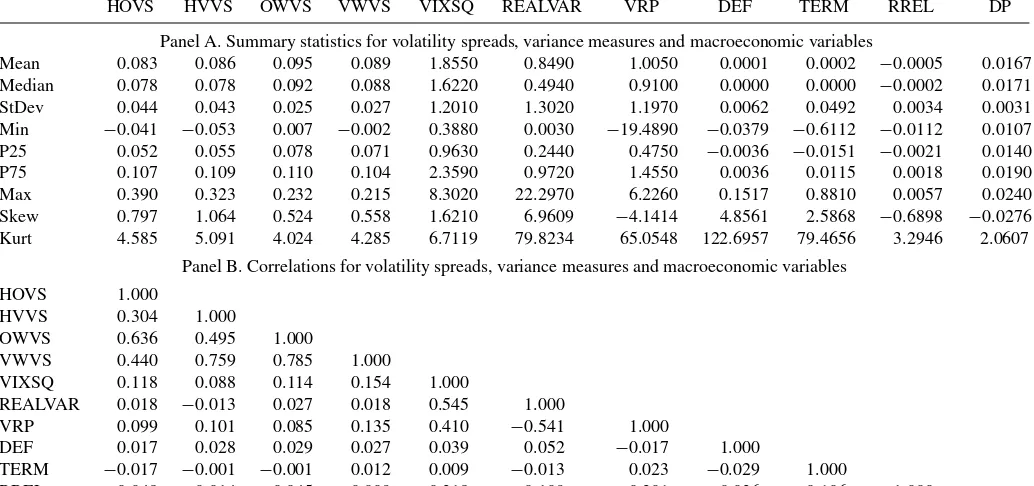
The descriptive statistics for the volatility spread measures are presented in Panel A ofTable 1. The mean (median) volatility spreads vary between 8.3% and 9.5% (7.8% and 9.2%) indi-cating that, on average, S&P 500 index put options have about 8–9% higher volatility than index call options during our sample period. For the highest open interest- and highest volume-based volatility spread measures, the standard deviations are about half of the mean and median volatility spreads. For the open interest-and volume-weighted volatility spread measures, the stinterest-andard deviations are about a quarter of the mean and median volatility spreads. The skewness and kurtosis estimates of the volatility spread measures indicate that the volatility spreads are mildly right-skewed and extreme deviations from the median are rare. As reported in Panel B ofTable 1, the correlations between the implied volatility measures vary between 0.30 and 0.79.
The main measure used to control for the conditional volatil-ity in Equation (1) is VIXSQ. VIX is the implied volatil-ity which measures the market’s forecast of the volatilvolatil-ity of
(2006) also argued that ignoring the nonsynchronicity between the option and stock markets can bias empirical results. We take this issue into account by skipping the overnight returns to calculate one-period ahead market returns.
the S&P 500 index and is obtained from the Chicago Board Options Exchange (CBOE). VIX is computed from the Eu-ropean style S&P 500 index option prices and incorporates information from the volatility smile by using a wide range of strike prices. The implied variance denoted by VIXSQ is equal to the square of VIX. In some specifications, we use an alternative measure of conditional volatility, realized variance (REALVAR), calculated as the sum of squared five-minute re-turns adjusted for fifth-order autocorrelation as in Andersen et al. (2001).4The intraday price data are obtained from Olsen Data Corporation.5 Panel A of Table 1 shows that the daily means (medians) are 1.86 (1.62) and 0.85 (0.49) in percentages squared terms for VIXSQ and REALVAR, respectively. VIXSQ exhibits mild skewness and kurtosis, whereas the deviations from normality are more extreme for REALVAR. The correla-tion between daily (monthly) implied and realized volatility is 0.55 (0.81).
Furthermore, to make sure that our results are not affected by model misspecification, we add a set of control variables (Xt)
that are expected to have a predictive relation with the excess market return.6 DEF is the change in the default spread cal-culated as the change in the difference between the yields on BAA- and AAA-rated corporate bonds. TERM is the change in the term spread calculated as the change in the difference between the yields on the 10-year Treasury bond and one-month Treasury bill. RREL is the detrended riskless rate de-fined as the yield on the one-month Treasury bill minus its one-year backward moving average.7 DP is the dividend-to-price ratio calculated by using the returns on the S&P 500 index with and without dividends. Finally, we include the lagged re-turn on the index, RET, to control for the serial correlation in market returns. The set of macroeconomic controls used in re-gressions changes as the measurement window of the expected market returns changes. We measure DEF and TERM as the change in the default and term premia over the last period, RET as the return over the last period and RREL and DP as the
4We use this autocorrelation adjustment to control for the microstructure noise
in high-frequency returns. Blume and Stambaugh (1983) showed that zero-mean noise in prices leads to strictly positive bias in zero-mean returns. Similarly, Asparouhova, Bessembinder, and Kalcheva (2013) investigated how noisy prices can impart bias to mean return estimates and regression parameters. Bandi and Russell (2006) and Andersen, Bollerslev, and Meddahi (2011) studied the impact of noisy prices on realized volatility estimates. We base our realized variance measures on varying past five-minute return windows according to the forecasting horizon. For example, when we forecast one-month ahead returns, we base our realized variance measure on the summation of the within-day five-minute squared returns over the preceding month adjusted for fifth-order serial correlation.
5At an earlier stage of the study, we also use RANGEVAR, the range volatility
defined as the square of the difference between the logarithm of the highest price and the logarithm of the lowest price in each period. As discussed by Brandt and Diebold (2006), range volatility is highly efficient, robust to microstructural noise and approximately Gaussian. All results presented in the article also hold for range volatility and they are available upon request.
6See, for example, Keim and Stambaugh (1986), Campbell (1987), Campbell
and Shiller (1988), Fama and French (1988,1989), Harvey (1989), and Ferson and Harvey (1991,1999).
7The time-series data on daily 10-year Treasury bond yields and BAA- and
AAA-rated corporate bond yields are available at the Federal Reserve statistical release web site. Daily yields on the one-month Treasury bill are downloaded from Kenneth French’s online data library.
Table 1. Descriptive statistics
HOVS HVVS OWVS VWVS VIXSQ REALVAR VRP DEF TERM RREL DP
Panel A. Summary statistics for volatility spreads, variance measures and macroeconomic variables
Mean 0.083 0.086 0.095 0.089 1.8550 0.8490 1.0050 0.0001 0.0002 −0.0005 0.0167 Median 0.078 0.078 0.092 0.088 1.6220 0.4940 0.9100 0.0000 0.0000 −0.0002 0.0171 StDev 0.044 0.043 0.025 0.027 1.2010 1.3020 1.1970 0.0062 0.0492 0.0034 0.0031 Min −0.041 −0.053 0.007 −0.002 0.3880 0.0030 −19.4890 −0.0379 −0.6112 −0.0112 0.0107 P25 0.052 0.055 0.078 0.071 0.9630 0.2440 0.4750 −0.0036 −0.0151 −0.0021 0.0140 P75 0.107 0.109 0.110 0.104 2.3590 0.9720 1.4550 0.0036 0.0115 0.0018 0.0190 Max 0.390 0.323 0.232 0.215 8.3020 22.2970 6.2260 0.1517 0.8810 0.0057 0.0240 Skew 0.797 1.064 0.524 0.558 1.6210 6.9609 −4.1414 4.8561 2.5868 −0.6898 −0.0276 Kurt 4.585 5.091 4.024 4.285 6.7119 79.8234 65.0548 122.6957 79.4656 3.2946 2.0607
Panel B. Correlations for volatility spreads, variance measures and macroeconomic variables HOVS 1.000
HVVS 0.304 1.000
OWVS 0.636 0.495 1.000
VWVS 0.440 0.759 0.785 1.000
VIXSQ 0.118 0.088 0.114 0.154 1.000
REALVAR 0.018 −0.013 0.027 0.018 0.545 1.000
VRP 0.099 0.101 0.085 0.135 0.410 −0.541 1.000
DEF 0.017 0.028 0.029 0.027 0.039 0.052 −0.017 1.000
TERM −0.017 −0.001 −0.001 0.012 0.009 −0.013 0.023 −0.029 1.000
RREL 0.048 0.014 0.045 0.009 −0.318 −0.109 −0.201 −0.036 −0.106 1.000
DP −0.006 0.001 −0.062 −0.027 −0.253 −0.093 −0.153 0.018 −0.005 0.022 1.000
NOTE: This table presents descriptive statistics for various volatility spread measures, implied variance, realized variance, volatility risk premium, and macroeconomic variables. Panel A presents the summary statistics for volatility spreads, variance measures, and macroeconomic variables. Panel B presents the correlation matrix between the volatility spreads, variance measures, and macroeconomic control variables. HOVS (HVVS) is the implied volatility difference between the OTM put option and the ATM call option that have the highest open interest (volume) in a given trading day. VWVS (OWVS) is equal to the difference between the volume-weighted (open interest-weighted) average of the volatility spreads for all OTM put options and the volume-weighted (open interest-weighted) average of the volatility spreads for all ATM call options. VIXSQ is the implied variance which measures the market’s forecast of the volatility of the S&P 500 index. REALVAR is the realized variance calculated as the sum of squared five-minute returns adjusted for fifth-order autocorrelation. VRP is the volatility risk premium defined as the difference between VIXSQ and REALVAR. DEF is the change in the default spread calculated as the change in the difference between the yields of BAA- and AAA-rated corporate bonds. TERM is the change in the term spread calculated as the change in the difference between the yields of the 10-year Treasury bond and the one-month Treasury bill. RREL is the detrended riskless rate defined as the one-month Treasury bill rate minus its one-year backward moving average. DP is the aggregate dividend price ratio obtained by using the S&P 500 index return with and without dividends.
detrended riskless rate and the dividend-to-price ratio at the end of the last period. Panel B ofTable 1 shows that there is no strong correlation between the volatility spread measures and the macroeconomic control variables. For daily (monthly) data, theR2from a contemporaneous regression of volatility spreads on implied variance and the macroeconomic variables is about 3.00% (4.66%).
3. EMPIRICAL RESULTS
3.1 Intertemporal Relation Between Volatility Spreads
and Market Returns
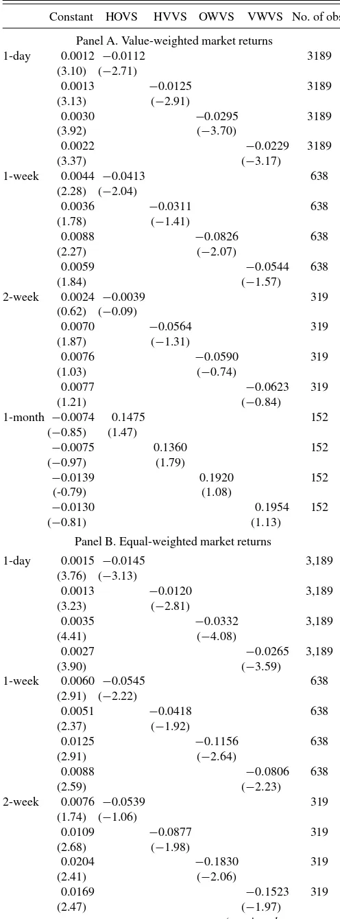
Table 2presents results from the univariate time-series regres-sions of one-period ahead excess returns of the S&P 500 index on various volatility spread measures. In Panel A (Panel B), the dependent variable is the one-day, one-week, two-week, and one-month ahead value-weighted (equal-weighted) excess returns on the S&P 500 index. The first row in each regres-sion gives the intercepts and slope coefficients. The second row presents the Newey and West (1987) adjustedt-statistics using optimal lag length.8
8Following Newey and West (1994), we use automatic lag length selection in
the covariance matrix estimation of Newey and West (1987) standard errors. Newey and West (1994) employed a nonparametric approach (a truncated
ker-The first set of results inTable 2 pertain to the regression of one-day ahead excess market returns on the lagged volatility spreads. The results show that all volatility spread measures have significantly negative coefficients, reflecting the fact that when put options are relatively more expensive with respect to call options written on the S&P 500 index, one-day ahead market returns are expected to be lower. This is consistent with the idea that investors with favorable (unfavorable) expectations about future index movements will buy more call (put) options before price increases (decreases). For the value-weighted returns in Panel A, the coefficients of the volatility spread measures range from −0.0112 to −0.0295, implying considerable economic significance as well. When volatility spreads increase by 1%, one-day ahead excess market returns decrease by 1.12 to 2.95 basis points, which corresponds to 2.82%–7.43% per annum assuming 252 trading days in a year. Moreover, the Newey and Westt-statistics are high in absolute magnitude ranging from −2.71 (for HOVS) to−3.70 (for OWVS). Hence, we observe both economically and statistically significant parameter esti-mates. For the equal-weighted returns in Panel B, the results are even stronger. The coefficients of the volatility spread measures range from−0.0120 to −0.0332 and the t-statistics for these coefficients are between−2.81 and−4.08.
nel estimator) to estimating the optimal bandwidth from the data, rather than specifying a value a priori.
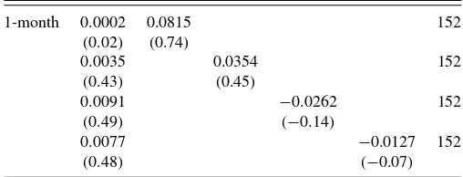
Second set of regressions in both panels test weekly pre-dictability using nonoverlapping weekly observations. For the value-weighted returns in Panel A, the coefficients of the volatility spread measures are still significantly negative rang-ing from−0.0311 to−0.0826. In other words, when volatility spread measures increase by 1%, one-week ahead aggregate stock returns decrease by 3.11 to 8.26 basis points. However, two of the four volatility spread measures are not significant at conventional levels. When we focus on equal-weighted market returns in Panel B, we find that all volatility spread measures have a significantly negative relation with expected weekly mar-ket returns. The coefficient estimates are between−0.0418 and −0.1156 and the correspondingt-statistics are between−1.92 and−2.64. Extending the measurement window for expected market returns to nonoverlapping two weeks or one month takes away significance of the slope coefficients on volatility spread measures. For the value-weighted returns, at the two-week horizon, the coefficient of HOVS (HVVS) has the low-est (highlow-est) statistical significance with at-statistic of −0.09 (−1.31), whereas for the one-month horizon, the coefficients of the volatility spread measures become positive but they are still insignificant. For the equal-weighted returns reported in Panel B, although we observe some significantly negative coefficients at the two-week horizon, the results are qualitatively similar to those reported for the value-weighted returns in Panel A. Col-lectively, these results suggest that there is an economically and statistically significant relation between volatility spreads and market returns and this predictability extends to a weekly hori-zon. We believe that the weekly predictability that the results indicate is consistent with our information-based explanation as option and equity markets typically assimilate information quickly and it is not likely that it would take more than one week for any information revealed in the option market to be reflected in the stock market.
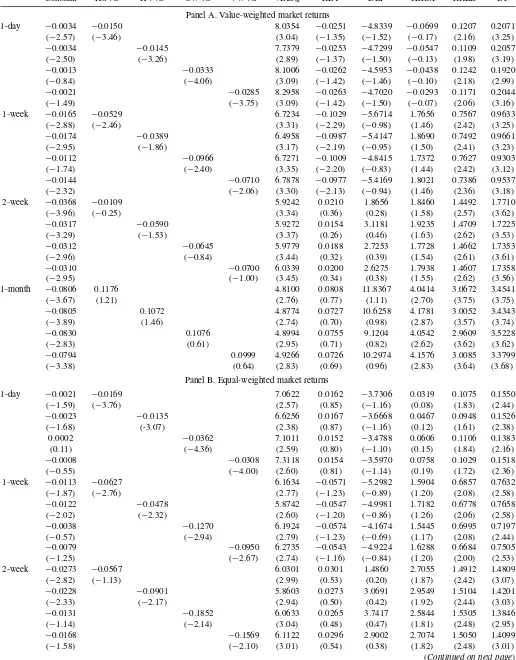
Table 3presents results from the multivariate time-series re-gressions of one-period ahead excess returns of the S&P 500 index on various volatility spread measures and control vari-ables as in Equation (1). We expect to find significantly positive slope coefficients for the conditional variance measures as doc-umented by Bali and Peng (2006) at the daily frequency and Guo and Whitelaw (2006) at the monthly frequency. We also control for various macroeconomic variables. Again, Panels A and B present results for value- and equal-weighted expected market returns, respectively.
The daily regressions in both panels show that the negative relation between volatility spreads and excess market returns is robust to the inclusion of the control variables in the regression specifications. Thet-statistics for the volatility spreads vary be-tween−3.26 and−4.06 for value-weighted returns and−3.07 and−4.36 for equal-weighted returns. The weekly predictability documented inTable 2also extends to the multivariate setting. The volatility spread measures havet-statistics that range from −1.86 to −2.40 for value-weighted returns and from −2.32 to−2.94 for equal-weighted returns at the one-week horizon. Although three of the four volatility spread measures can fore-cast equal-weighted market returns at the two-week horizon as shown in Panel B ofTable 3, bi-weekly predictability does not exist for value-weighted returns. Neither panel displays any
Table 2. Volatility spreads and market returns: Univariate regressions
Constant HOVS HVVS OWVS VWVS No. of obs.
Panel A. Value-weighted market returns
(continued on next page)
Table 2. Volatility spreads and market returns: Univariate
NOTE: This table presents parameter estimates from the time-series predictive regressions of excess returns of the S&P 500 index on volatility spreads. Panel A presents results for the value-weighted market returns and Panel B presents results for the equal-weighted market returns. Volatility spread measures are defined inTable 1. In each regression, the dependent variable is the 1-day, 1-week, 2-week, or 1-month excess market returns, where the returns start accruing from the opening of the next trading day. For each regression, the first row gives the intercepts and slope coefficients. The second row presents Newey–West adjusted
t-statistics using optimal lag length. The last column reports the number of nonoverlapping observations used in predictive regressions.
predictive power of volatility spreads for monthly excess mar-ket returns. To summarize, with the addition of the macroeco-nomic variables, the noise in the index returns is reduced and, if anything, the negative relation between volatility spreads and expected market returns becomes even stronger.
Going forward, we only report results for value-weighted returns both to be more conservative and to take into account the possibility that equal-weighted returns are more sensitive to microstructure noise.
The results in Table 3also show that the implied variance measured by VIXSQ is positively and significantly related to one-period ahead excess S&P 500 returns.9In the regressions of one-day ahead excess market returns, the estimated coefficients on the lagged implied volatility are in the range of 7.74 and 8.30. The t-statistics associated with these coefficients range from 2.89 to 3.09. When the excess returns are extended to longer horizons, VIXSQ remains a significant predictor of fu-ture returns. One can also see that the estimated coefficients on the dividend-to-price ratio and the detrended riskless rate are significantly positive. Also, the change in the term premium is significant for the one-month horizon.
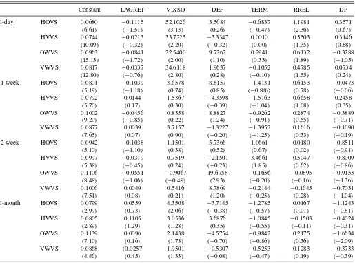
Next, we answer the question whether expected market re-turns can predict the volatility spread measures, or in other words, whether the predictability runs the other way around. Table 4presents results from the regressions of one-period ahead volatility spread measures on the value-weighted excess S&P index returns, implied variance and macroeconomic variables. The results show that the lagged stock returns computed using windows ranging from one day to one month cannot predict volatility spreads. Thet-statistics for the coefficients of lagged daily returns vary from−0.32 to−1.72 and thet-statistics for the coefficients of lagged monthly returns vary from 0.16 to 1.29. None of the control variables can forecast volatility spreads with the exception of VIXSQ that has a significantly positive relation with future volatility spreads at the daily horizon. Although not reported in the article to save space, similar results are obtained
9The significantly positive relation between implied variances and expected
market returns also holds for the realized and range variances, and they are available upon request.
without controlling for implied variance (VIXSQ) and macroe-conomic variables, that is, lagged market returns do not predict future volatility spreads.
These results collectively suggest that the implied volatility spreads can predict aggregate equity returns up to a one-week horizon; however, there is no predictability in the opposite di-rection.
3.2 Controlling for Variance Risk Premium
Bollerslev, Tauchen, and Zhou (2009) argued that the long-run risk in consumption growth is a fundamental determinant of the equity premium and dynamic dependencies among as-set returns over the long-run. Bollerslev, Tauchen, and Zhou (2009) showed that the variance risk premium, defined as the difference between expected variance under the risk-neutral measure and expected variance under the physical measure, predicts future market returns, especially at the quarterly horizon.
Our volatility spread measure is constructed as the differ-ence between the volatilities of OTM put options and ATM call options written on the S&P 500 index. As such, it is a differ-ence between two market volatility measures and is potentially correlated with the variance risk premium. To ensure that our results are not driven by a correlation between implied volatility spreads and variance risk premium, we first test a generalized version of the specification in Bollerslev, Tauchen, and Zhou (2009) and include both the implied variance and the realized variance in the regressions:
Rt+1=α+βVSt+γVIXSQt+δREALVARt+θ Xt+εt+1. (2)
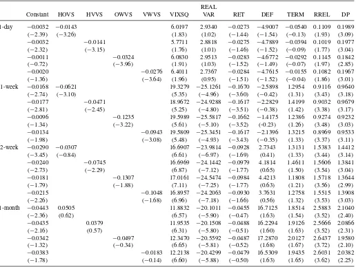
The results are presented inTable 5. First set of regressions show that, at the daily forecasting horizon, all four volatil-ity spread measures have significantly negative coefficients in the presence of VIXSQ and REALVAR in the specification. The coefficients vary between−0.0141 and−0.0324 and the
t-statistics vary between −3.15 and −3.96. Due to the high correlation between VIXSQ and REALVAR, both conditional volatility measures lose their significance albeit retaining their positive coefficients. Extending the forecasting horizon to one week indicates that the significantly negative relation between volatility spreads and expected market returns continues to hold. Thet-statistics associated with the coefficients of the volatility spread measures range from−2.45 and −3.22 at the weekly horizon. At the two-week and one-month horizons, there is no robust relation between volatility spreads and expected market returns. Also, the high correlation between VIXSQ and REAL-VAR becomes more pronounced at return horizons longer than one day. This multicollinearity problem causes VIXSQ to have a higher and more significantly positive coefficient compared to earlier specifications in which VIXSQ is the only variance proxy. Moreover, the coefficient of REALVAR turns negative and becomes highly significant, whereas it is significantly pos-itive when included in the specification in isolation.
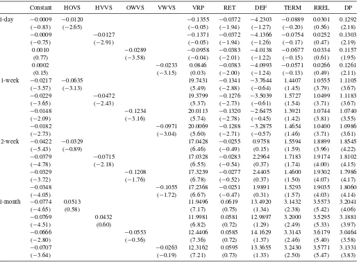
InTable 6, we include the variance risk premium, denoted as VRP, directly in the regressions.
Rt+1=α+βVSt+γVRPt+θ Xt+εt+1. (3)
Table 3. Volatility spreads and market returns: Multivariate regressions
Constant HOVS HVVS OWVS VWVS VIXSQ RET DEF TERM RREL DP
Panel A. Value-weighted market returns
1-day −0.0034 −0.0150 8.0354 −0.0251 −4.8339 −0.0699 0.1207 0.2071 (−2.57) (−3.46) (3.04) (−1.35) (−1.52) (−0.17) (2.16) (3.25)
−0.0034 −0.0145 7.7379 −0.0253 −4.7299 −0.0547 0.1109 0.2057 (−2.50) (−3.26) (2.89) (−1.37) (−1.50) (−0.13) (1.98) (3.19)
−0.0013 −0.0333 8.1006 −0.0262 −4.5953 −0.0438 0.1242 0.1920 (−0.84) (−4.06) (3.09) (−1.42) (−1.46) (−0.10) (2.18) (2.99) −0.0021 −0.0285 8.2958 −0.0263 −4.7020 −0.0293 0.1171 0.2044
(−1.49) (−3.75) (3.09) (−1.42) (−1.50) (−0.07) (2.06) (3.16) 1-week −0.0165 −0.0529 6.7234 −0.1029 −5.6714 1.7656 0.7567 0.9633
(−2.88) (−2.46) (3.31) (−2.29) (−0.98) (1.46) (2.42) (3.25)
−0.0174 −0.0389 6.4958 −0.0987 −5.4147 1.8690 0.7492 0.9661 (−2.95) (−1.86) (3.17) (−2.19) (−0.95) (1.50) (2.41) (3.23)
−0.0112 −0.0966 6.7271 −0.1009 −4.8415 1.7372 0.7627 0.9303 (−1.74) (−2.40) (3.35) (−2.20) (−0.83) (1.44) (2.42) (3.12)
−0.0144 −0.0710 6.7878 −0.0977 −5.4169 1.8021 0.7386 0.9537 (−2.32) (−2.06) (3.30) (−2.13) (−0.94) (1.46) (2.36) (3.18) 2-week −0.0368 −0.0109 5.9242 0.0210 1.8656 1.8460 1.4492 1.7710
(−3.96) (−0.25) (3.34) (0.36) (0.28) (1.58) (2.57) (3.62)
−0.0317 −0.0590 5.9272 0.0154 3.1181 1.9235 1.4709 1.7225 (−3.29) (−1.53) (3.37) (0.26) (0.46) (1.63) (2.62) (3.53)
−0.0312 −0.0645 5.9779 0.0188 2.7253 1.7728 1.4662 1.7353 (−2.96) (−0.84) (3.44) (0.32) (0.39) (1.54) (2.61) (3.61)
−0.0310 −0.0700 6.0339 0.0200 2.6275 1.7938 1.4607 1.7358 (−2.95) (−1.00) (3.45) (0.34) (0.38) (1.55) (2.62) (3.56) 1-month −0.0806 0.1176 4.8100 0.0808 11.8367 4.0414 3.0672 3.4541
(−3.67) (1.21) (2.76) (0.77) (1.11) (2.70) (3.75) (3.75)
−0.0805 0.1072 4.8774 0.0727 10.6258 4.1781 3.0052 3.4343 (−3.89) (1.46) (2.74) (0.70) (0.98) (2.87) (3.57) (3.74)
−0.0830 0.1076 4.8994 0.0755 9.1204 4.0542 2.9609 3.5228 (−2.83) (0.61) (2.95) (0.71) (0.82) (2.62) (3.62) (3.62)
−0.0794 0.0999 4.9266 0.0726 10.2974 4.1576 3.0085 3.3799
(−3.38) (0.64) (2.83) (0.69) (0.96) (2.83) (3.64) (3.68) Panel B. Equal-weighted market returns
1-day −0.0021 −0.0169 7.0622 0.0162 −3.7306 0.0319 0.1075 0.1550 (−1.59) (−3.76) (2.57) (0.85) (−1.16) (0.08) (1.83) (2.44)
−0.0023 −0.0135 6.6256 0.0167 −3.6668 0.0467 0.0948 0.1526 (−1.68) (-3.07) (2.38) (0.87) (−1.16) (0.12) (1.61) (2.38)
0.0002 −0.0362 7.1011 0.0152 −3.4788 0.0606 0.1106 0.1383
(0.11) (−4.36) (2.59) (0.80) (−1.10) (0.15) (1.84) (2.16)
−0.0008 −0.0308 7.3118 0.0154 −3.5970 0.0758 0.1029 0.1518 (−0.55) (−4.00) (2.60) (0.81) (−1.14) (0.19) (1.72) (2.36) 1-week −0.0113 −0.0627 6.1634 −0.0571 −5.2982 1.5904 0.6857 0.7632
(−1.87) (−2.76) (2.77) (−1.23) (−0.89) (1.20) (2.08) (2.58)
−0.0122 −0.0478 5.8742 −0.0547 −4.9981 1.7182 0.6778 0.7658 (−2.02) (−2.32) (2.60) (−1.20) (−0.86) (1.26) (2.06) (2.58)
−0.0038 −0.1270 6.1924 −0.0574 −4.1674 1.5445 0.6995 0.7197 (−0.57) (−2.94) (2.79) (−1.23) (−0.69) (1.17) (2.08) (2.44) −0.0079 −0.0950 6.2735 −0.0543 −4.9224 1.6288 0.6684 0.7505
(−1.25) (−2.67) (2.74) (−1.16) (−0.84) (1.20) (2.00) (2.53) 2-week −0.0273 −0.0567 6.0301 0.0301 1.4860 2.7055 1.4912 1.4809
(−2.82) (−1.13) (2.99) (0.53) (0.20) (1.87) (2.42) (3.07)
−0.0228 −0.0901 5.8603 0.0273 3.0691 2.9549 1.5104 1.4201 (−2.33) (−2.17) (2.94) (0.50) (0.42) (1.92) (2.44) (3.03)
−0.0131 −0.1852 6.0633 0.0265 3.7417 2.5844 1.5305 1.3846 (−1.14) (−2.14) (3.04) (0.48) (0.47) (1.81) (2.48) (2.95)
−0.0168 −0.1569 6.1122 0.0296 2.9002 2.7074 1.5050 1.4099 (−1.58) (−2.10) (3.01) (0.54) (0.38) (1.82) (2.48) (3.01)
(Continued on next page)
Table 3. Volatility spreads and market returns: Multivariate regressions (Continued)
1-month −0.0639 0.0406 5.1414 0.0771 8.4209 4.3259 3.0738 2.8720
(−2.43) (0.40) (2.81) (0.66) (0.82) (2.57) (3.07) (2.82)
−0.0607 0.0018 5.2674 0.0756 8.1065 4.4108 3.0786 2.8382 (−2.50) (0.02) (2.72) (0.65) (0.80) (2.64) (3.08) (2.83)
−0.0419 −0.1670 5.6950 0.0728 10.8117 4.7787 3.2654 2.5669 (−1.27) (−0.92) (3.11) (0.64) (0.97) (2.74) (3.30) (2.47)
−0.0505 −0.1194 5.5567 0.0755 8.7389 4.5688 3.1635 2.7989 (−1.88) (−0.79) (2.93) (0.66) (0.85) (2.73) (3.27) (2.88)
NOTE: This table presents parameter estimates from the time-series predictive regressions of excess returns of the S&P 500 index on volatility spreads, implied variance, and macroeconomic variables. Volatility spread measures, implied variance, and macroeconomic variables are defined inTable 1. Panel A presents results for the value-weighted market returns and Panel B presents results for the equal-weighted market returns. In each regression, the dependent variable is the 1-day, 1-week, 2-week, or 1-month ahead excess market returns, where the returns start accruing from the opening of the next trading day. For each regression, the first row gives the intercepts and slope coefficients. The second row presents Newey–West adjustedt-statistics using optimal lag length.
The correlation between VRP and VIXSQ is 0.83 and the correlation between VRP and REALVAR is 0.36 at the monthly frequency, in line with the findings of Bollerslev, Tauchen, and Zhou (2009). The correlation between the variance risk pre-mium and our implied volatility measures range from 0.09 and 0.14 (0.12 and 0.19) at the daily (monthly) frequency indicating
that the two types of measures capture different information. Supporting this finding, all the volatility spread measures have significantly negative coefficients up to a return forecasting hori-zon of one week. Thet-statistics associated with the coefficients of the volatility spreads range from−2.65 to−3.58 at the one-day horizon and from−2.43 to−3.16 at the one-week horizon.
Table 4. Market returns predicting volatility spreads
Constant LAGRET VIXSQ DEF TERM RREL DP
1-day HOVS 0.0680 −0.1115 52.1026 3.5684 −0.6837 1.1981 0.3571 (6.61) (−1.51) (3.13) (0.26) (−0.47) (2.36) (0.67) HVVS 0.0744 −0.0213 33.7225 −3.3347 0.0010 0.5503 0.3146
(10.09) (−0.32) (2.20) (−0.32) (0.00) (1.35) (0.88) OWVS 0.0963 −0.0841 22.5400 9.7262 0.2941 0.6132 −0.3288
(15.13) (−1.72) (2.00) (1.10) (0.33) (1.89) (−1.05) VWVS 0.0817 −0.0337 34.6118 1.9637 −0.1052 0.4785 0.0734
(12.80) (−0.76) (2.80) (0.28) (−0.10) (1.55) (0.24) 1-week HOVS 0.0801 −0.1039 3.6578 8.8157 −1.4131 0.6153 −0.0473
(5.19) (−1.18) (0.74) (0.85) (−0.88)) (0.78) (−0.06) HVVS 0.0792 0.0144 1.5367 −4.3598 −1.5163 0.6658 0.2458
(5.70) (0.17) (0.30) (−0.39) (−1.04) (1.08) (0.35)
OWVS 0.1002 −0.0456 0.8358 8.8827 −0.9262 0.2874 −0.3889 (9.20) (−0.85) (0.22) (1.24) (−0.91) (0.55) (−0.71) VWVS 0.0877 0.0039 3.7157 −1.3227 −1.3952 0.1616 −0.1090 (7.65) (0.07) (0.90) (−0.20) (−1.25) (0.33) (−0.19) 2-week HOVS 0.0942 −0.1038 1.1501 5.7366 1.0661 0.0180 −0.8511 (5.10) (−1.10) (0.38) (0.52) (0.67) (0.02) (−0.91) HVVS 0.0997 −0.0319 0.7519 −2.1501 3.4661 0.5047 −0.8009 (5.38) (−0.45) (0.24) (−0.23) (1.85) (0.62) (−0.86) OWVS 0.1106 −0.0551 −0.9067 19.6758 −0.1656 −0.0895 −0.9153 (8.48) (−1.06) (−0.49) (2.93) (−0.20) (−0.16) (−1.36) VWVS 0.1006 0.0049 0.5416 8.7869 −0.2144 −0.1645 −0.7031 (7.51) (0.08) (0.21) (1.20) (−0.25) (0.28) (−1.04) 1-month HOVS 0.0799 0.0559 4.3508 −3.7145 −1.2785 0.0167 −1.1243 (2.99) (0.73) (2.06) (−0.38) (−0.57) (0.01) (−0.81) HVVS 0.0805 0.1105 3.0536 3.6876 −1.0845 −0.1503 −0.4024 (2.89) (1.29) (1.28) (0.35) (−0.55) (−0.11) (−0.31)
OWVS 0.1139 0.0096 2.1438 −4.5754 −0.9842 0.2175 −1.6634 (7.10) (0.16) (1.73) (−0.70) (−0.86) (0.36) (−2.09) VWVS 0.0868 (0.0257 1.9501 −0.5307 −0.5253 0.1283 −0.3733 (4.46) (0.45) (1.33) (−0.08) (−0.47) (0.19) (−0.39)
NOTE: This table presents parameter estimates from the time-series predictive regressions of one-period ahead volatility spreads on the value-weighted excess S&P 500 index returns, implied variance and macroeconomic variables. Volatility spread measures, implied variance and macroeconomic variables are defined inTable 1. In each regression, the dependent variable is the 1-day, 1-week, 2-week, or 1-month ahead volatility spreads. For each regression, the first row gives the intercepts and slope coefficients. The second row presents Newey–West adjustedt-statistics using optimal lag length.
Table 5. Controlling for variance risk premium
REAL
Constant HOVS HVVS OWVS VWVS VIXSQ VAR RET DEF TERM RREL DP
1-day −0.0032 −0.0143 6.0197 2.9340 −0.0273 −4.9007 −0.0540 0.1109 0.1989 (−2.39) (−3.26) (1.83) (1.02) (−1.44) (−1.54) (−0.13) (1.93) (3.09)
−0.0032 −0.0141 5.7711 2.8818 −0.0275 −4.7889 −0.0394 0.1019 0.1977 (−2.32) (−3.15) (1.76) (1.01) (−1.46) (−1.52) (−0.09) (1.77) (3.04)
−0.0011 −0.0324 6.0830 2.9513 −0.0283 −4.6772 −0.0292 0.1145 0.1842 (−0.72) (−3.96) (1.91) (1.03) (−1.52) (−1.49) (−0.07) (1.97) (2.85)
−0.0020 −0.0276 6.4011 2.7367 −0.0284 −4.7615 −0.0155 0.1082 0.1967 (−1.36) (−3.64) (1.96) (0.95) (−1.51) (−1.52) (−0.04) (1.86) (3.01) 1-week −0.0168 −0.0621 19.3279 −25.1261 −0.1670 −2.5898 1.2954 0.9116 0.9640
(−2.74) (−3.10) (5.35) (−4.96) (−3.60) (−0.42) (1.31) (3.43) (3.18)
−0.0177 −0.0471 18.9672 −24.9288 −0.1617 −2.2829 1.4199 0.9032 0.9679 (−2.81) (−2.45) (5.25) (−4.80) (−3.51) (−0.38) (1.42) (3.38) (3.17) −0.0096 −0.1235 19.5989 −25.5817 −0.1662 −1.4175 1.2386 0.9274 0.9232
(−1.34) (−3.22) (5.61) (−5.10) (−3.52) (-0.23) (1.26) (3.48) (3.03)
−0.0134 −0.0943 19.5809 −25.3451 −0.1617 −2.1396 1.3215 0.8969 0.9533 (−1.98) (−3.08) (5.48) (−4.93) (−3.43) (−0.35) (1.33) (3.37) (3.11) 2-week −0.0290 −0.0307 16.6907 −23.9814 −0.0928 2.7343 1.3131 1.5383 1.4412
(−3.45) (−0.84) (6.61) (−6.97) (−1.69) (0.41) (1.33) (3.44) (3.14)
−0.0240 −0.0745 16.6969 −24.1442 −0.0979 4.1814 1.4611 1.5606 1.3841 (−2.73) (−2.29) (6.87) (−7.12) (−1.77) (0.65) (1.50) (3.54) (3.04)
−0.0181 −0.1307 17.0161 −24.5474 −0.0984 4.4213 1.1808 1.5718 1.3644 (−1.79) (−1.88) (7.11) (−7.25) (−1.77) (0.63) (1.21) (3.56) (2.99)
−0.0215 −0.1048 16.8957 −24.2063 −0.0930 3.7631 1.2758 1.5515 1.3908 (−2.26) (−1.68) (6.96) (−7.18) (−1.66) (0.56) (1.32) (3.53) (3.03) 1-month −0.0443 0.0505 11.8832 −20.1011 −0.0455 16.7125 1.8514 2.5883 2.1040
(−2.36) (0.62) (6.57) (−5.90) (−0.47) (1.63) (1.54) (3.52) (2.40)
−0.0435 0.0379 11.9535 −20.1508 −0.0488 16.2294 1.9126 2.5666 2.0866 (−2.16) (0.57) (6.31) (−5.80) (−0.51) (1.60) (1.63) (3.52) (2.31) −0.0342 −0.0497 12.3470 −20.5592 −0.0487 17.2870 2.0127 2.6437 1.9580
(−1.32) (−0.34) (6.65) (−5.81) (−0.52) (1.68) (1.67) (3.72) (2.10)
−0.0383 −0.0183 12.2138 −20.4299 −0.0479 16.5309 1.9435 2.6031 2.0382 (−1.78) (−0.14) (6.60) (−5.88) (−0.50) (1.63) (1.65) (3.62) (2.25)
NOTE: This table presents parameter estimates from the time-series predictive regressions of excess returns of the S&P 500 index on volatility spreads, implied variance, realized variance, and macroeconomic variables. Volatility spread measures, implied variance, realized variance, and macroeconomic variables are defined inTable 1. In each regression, the dependent variable is the 1-day, 1-week, 2-week, or 1-month ahead excess value-weighted market returns, where the returns start accruing from the opening of the next trading day. For each regression, the first row gives the intercepts and slope coefficients. The second row presents Newey–West adjustedt-statistics using optimal lag length.
The coefficients of VRP indicate a significantly positive intertemporal relation between variance risk premia and excess market returns starting from the one-week horizon complement-ing the results of Bollerslev, Tauchen, and Zhou (2009).
3.3 Out-of-Sample Evidence and Economic
Significance
Goyal and Welch (2008) examined the performance of a wide variety of factors that have been suggested by the literature to be significant predictors of the equity premium. Their conclusion is that the in-sample performance of many of these predictors is weak. Moreover, the out-of-sample performance of the pre-dictors indicates that they would not have helped investors to profitably time the market. Hence, we need to investigate the out-of-sample significance of the volatility spread measures by simulating the return of a trading strategy which invests on the market portfolio or the risk-free asset. Yet another issue is the significance of trading costs. Since our findings suggests a straightforward mispricing, we need to understand if the pre-dictability is big enough to exceed transaction cost bounds.
To be able to address the issues of out-of-sample predictabil-ity and transaction cost bounds, we use a rolling window trading analysis. The trading strategy uses the out-of-sample one step ahead forecasts of the excess market return using one of our volatility spread measures, namely VWVS. The first forecasting regression uses the first half of the sample, that is, the first regres-sion uses the first 1593 observations of the overall sample and then the one-step ahead estimations use an expanding window. Specifically, on each daytafter the midpoint of the dataset, the data available up to daytare used to estimate our baseline pre-dictive regression. The estimated coefficients are recorded and used to forecast the excess market return at timet +1. Then for each dayt, the investment strategy invests 100% in the equity in-dex if the forecasted excess market return is positive or it invests 100% on the risk free rate if the forecasted excess return is neg-ative. On dayt + 1, the return of this portfolio is realized and a new cycle of predictive regressions is estimated using an ex-panded window. We denote this strategy as the optimal strategy. Consequently, we obtain a time series of returns for this strategy. However, there are certain transaction costs when this switch-ing tradswitch-ing algorithm is used. One cost is the brokerage fees
Table 6. Controlling for variance risk premium
Constant HOVS HVVS OWVS VWVS VRP RET DEF TERM RREL DP
1-day −0.0009 −0.0120 −0.1355 −0.0372 −4.2303 −0.0889 0.0301 0.1292 (−0.83) (−2.65) (−0.05) (−1.94) (−1.27) (−0.20) (0.56) (2.18)
−0.0009 −0.0127 −0.1371 −0.0372 −4.1366 −0.0754 0.0252 0.1303 (−0.75) (−2.91) (−0.05) (−1.94) (−1.26) (−0.17) (0.47) (2.19)
0.0010 −0.0289 −0.0958 −0.0383 −4.0138 −0.0677 0.0334 0.1157 (0.77) (−3.58) (−0.04) (−2.01) (−1.22) (−0.15) (0.61) (1.95) 0.0002 −0.0233 0.0846 −0.0383 −4.0993 −0.0571 0.0266 0.1261
(0.15) (−3.15) (0.03) (−2.00) (−1.24) (−0.13) (0.49) (2.11) 1-week −0.0217 −0.0635 19.7431 −0.1341 −3.7644 1.4407 1.0555 1.1105
(−3.57) (−3.13) (5.49) (−2.88) (−0.64) (1.45) (3.79) (3.67)
−0.0229 −0.0472 19.3799 −0.1276 −3.5039 1.5727 1.0499 1.1183 (−3.65) (−2.43) (5.37) (−2.73) (−0.61) (1.54) (3.71) (3.67)
−0.0148 −0.1234 20.0113 −0.1320 −2.6475 1.3921 1.0744 1.0740 (−2.09) (−3.16) (5.74) (−2.78) (−0.45) (1.42) (3.81) (3.55)
−0.0182 −0.0971 20.0069 −0.1288 −3.2875 1.4654 1.0400 1.0986 (−2.73) (−3.04) (5.60) (−2.71) (−0.57) (1.46) (3.71) (3.61)
2-week −0.0422 −0.0329 17.0428 −0.0255 0.9758 1.5594 1.8899 1.8545 (−5.43) (−0.89) (6.46) (−0.49) (0.15) (1.59) (3.96) (4.22)
−0.0379 −0.0715 17.0328 −0.0283 2.2964 1.7183 1.9174 1.8102 (−4.78) (−2.18) (6.55) (−0.54) (0.37) (1.74) (4.00) (4.15)
−0.0329 −0.1208 17.3239 −0.0277 2.4405 1.4600 1.9302 1.7986 (−3.72) (−1.76) (6.78) (−0.52) (0.37) (1.50) (4.07) (4.17)
−0.0348 −0.1055 17.2368 −0.0251 1.9891 1.5293 1.9035 1.8060 (−4.05) (−1.72) (6.67) (−0.47) (0.31) (1.57) (4.03) (4.14) 1-month −0.0774 0.0513 11.9496 0.0619 13.4920 3.1432 3.5573 3.2041
(−4.65) (0.58) (7.17) (0.75) (1.34) (2.38) (5.42) (4.06)
−0.0769 0.0432 11.9981 0.0581 12.9897 3.2000 3.5295 3.1881 (−4.51) (0.60) (6.82) (0.72) (1.29) (2.49) (5.33) (3.97)
−0.0666 −0.0553 12.4406 0.0585 14.1629 3.3143 3.6179 3.0464 (−2.80) (−0.36) (7.36) (0.72) (1.37) (2.46) (5.40) (3.58)
−0.0707 −0.0263 12.3162 0.0595 13.3655 3.2430 3.5771 3.1331 (−3.64) (−0.19) (7.21) (0.73) (1.33) (2.50) (5.47) (3.83)
NOTE: This table presents parameter estimates from the time-series predictive regressions of excess returns of the S&P 500 index on volatility spreads, volatility risk premium, and macroeconomic variables. Volatility spread measures, volatility risk premium, and macroeconomic variables are defined inTable 1. In each regression, the dependent variable is the 1-day, 1-week, 2-week, or 1-month ahead excess value-weighted market returns, where the returns start accruing from the opening of the next trading day. For each regression, the first row gives the intercepts and slope coefficients. The second row presents Newey–West adjustedt-statistics using optimal lag length.
and the other is the bid-ask spread. Exchange traded funds (ETFs) are popularly used to invest in market indices. There is a fixed brokerage fee when one invests in ETFs, which can be diluted by the amount invested in the fund since it is a fixed fee. In other words, the fee as a percentage of the investment decreases by the total amount invested. However, the bid-ask spreads are real costs that the switching investors need to bear. When we investigate the most famous ETF that invests in the S&P 500 index (ticker: SPY), we find that the bid-ask spread is 1 basis point. Hence, an investor bears this cost every time he/she switches between investments (in both directions). Therefore, after we find the optimal trading strategy, we decrease invest-ment returns by the bid-ask spread amount each time the strategy switches between investments.
We find that, when one allocates all his/her wealth to the eq-uity index portfolio, the strategy earns a daily return of 0.021%. This passive investment strategy has a Sharpe ratio of 0.020. To better understand this performance, we follow the growth path of an investment of $100 using this strategy and find that it grows to $129 by the end of the data period. When one invests in the optimal strategy, he/she earns an average daily return of
0.032% with a Sharpe ratio of 0.036. To compare the relative performance of the optimal strategy to the passive strategy of investing in the S&P 500 index, we track the growth of an in-vestment of $100 to the optimal strategy and find that it grows to $158 by the end of the estimation period. In other words, there is a significant difference between the optimal and the static portfolios. Finally, to be able to evaluate the effect of the bid-ask spreads, we identify the number of switching trades and decrease the optimal portfolio returns by the magnitude of the bid-ask spreads. This helps us to obtain the net optimal returns. We find that the optimal strategy yields a higher return compared to the passive strategy even after taking the bid-ask spreads into account. Specifically, the daily average return becomes 0.030% which corresponds to a Sharpe ratio of 0.033. An investment of
$100 into the optimal strategy grows to $151.6 after transaction costs are deducted. Hence, we conclude that even after taking the transaction costs into account, the optimal portfolio has a significantly better performance than the S&P 500 index itself both in a nominal sense and a risk-adjusted sense.
When we repeat the analysis for the other spread measures, we find qualitatively similar results.
4. INFORMATION EXPLANATION
4.1 Earnings Announcements
In this section, we provide additional evidence for the information-based explanation of the significant link between volatility spreads and future returns.10Admittedly, it is difficult to pinpoint periods of significant information releases that have the potential to impact the aggregate stock market. Neverthe-less, we focus on the earnings announcements of the firms that constitute the S&P 500 index motivated by the idea that earn-ings announcements are informationally intensive periods for individual firms and such informational events have the poten-tial to affect the aggregate stock market as well. Moreover, the earnings announcements of firms in the same industry tend to be clustered in time and this makes it easier to identify periods of significant information releases for empirical purposes.
We obtain the list of S&P 500 constituent firms from CRSP. The earnings announcement dates of these firms come from COMPUSTAT.11 If the negative relation between volatility spreads and aggregate returns is due to information flow from options to stock markets, we would expect this relation to be stronger during informationally intensive periods such as the earnings announcement periods of S&P 500 constituent firms. To test this hypothesis, we first define a dummy variable that is equal to one for a given trading day if a firm that is a constituent of the S&P 500 index makes an earnings announcement in that period and zero otherwise. Then, we estimate the following regression model for one-day ahead market returns:
Rt+1 =α+β1VSPLUSt+β2VSMINUSt+γVIXSQt
+θ Xt+εt+1, (4)
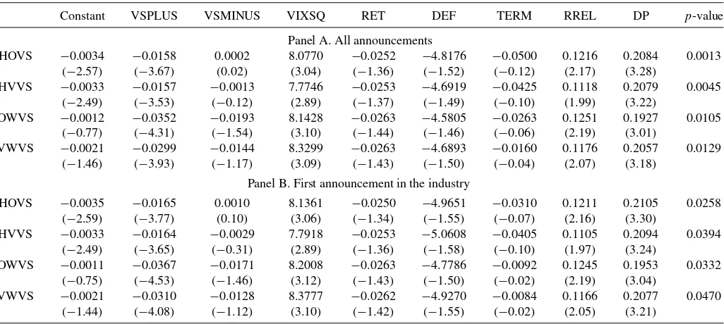
where VSPLUS is equal to the volatility spread if the dummy variable is equal to 1 and 0 otherwise; and VSMINUS is equal to the volatility spread if the dummy variable is equal to 0 and 0 otherwise. We expectβ1to be more negative (larger in absolute magnitude) thanβ2if the earnings announcements of S&P 500 constituent firms have an impact on the negative link between volatility spreads and excess market returns.
The coefficients of VSPLUS in Panel A ofTable 7vary be-tween−0.0157 and−0.0352. The lowestt-statistic in absolute magnitude is associated with HVVS and is equal to−3.53. On the other hand, the coefficients of VSMINUS are never signifi-cantly different from zero and thet-statistics range from−1.54 to 0.02. The last column presents thep-values associated with the Wald test for the equality of the coefficients of VSPLUS and VSMINUS. In all the specifications, VSPLUS is significantly more negative than VSMINUS such that thep-values are all lower than 2%. The fact that the predictive ability of volatility spreads for future market returns is constrained to the periods of earnings announcements by S&P 500 constituent firms lends
10Rather than drawing on the potential preference of informed traders for the
option market, the information explanation can also be supported by the idea that the option market incorporates available information to the prices more efficiently than the stock market. In this case, the mispricing in the stock market would lead to apparent volatility spreads in the options market, and the reversal of the mispricing would result in the predictive power of volatility spreads.
11The results are qualitatively similar when the earnings announcement dates
are collected from I/B/E/S.
support to the idea that the negative intertemporal relation be-tween volatility spreads and aggregate returns is driven by the trading activities of informed investors.
Next, we further refine the earnings announcement periods and focus on the first announcement done by an S&P 500 con-stituent firm in a given industry for a particular month. Specifi-cally, we define a dummy variable that is equal to one for a given trading day, if a firm that is a constituent of the S&P 500 index makes the first earnings announcement in a particular industry-month and accordingly estimate Equation (4). In this test, we are motivated by the idea that the first earnings announcement in an industry will have the most informational impact since the stock returns of the firms in the same industry tend to be cor-related. The results are presented in Panel B ofTable 7. Again, the coefficients of VSPLUS are significantly negative and their
t-statistics vary between−3.65 and−4.53. In contrast, the co-efficients of VSMINUS are statistically insignificant without any exception. Thep-values reported in the last column range from 2.58% to 4.70% and indicate that the predictive ability of volatility spreads for excess market returns is significantly stronger during periods of significant information releases by S&P 500 constituent firms.
4.2 Cash Flow and Expected Return News
It is well-known that three sources explain variation in stock returns: variation in expected returns, change in expected future cash flows (cash flow news), and change in expected future re-turns (expected return news). For example, Fama (1990), Schw-ert (1990), and others regressed stock returns on the change in cash flow variables. In these regressions, coefficient estimates and explained variances are considered to be a measure of how well those variables proxy for change in expected cash flows. However, as argued in the literature, explanatory power of cash flow proxies may arise from the correlation of cash flow proxies with expected returns, cash flow news and/or expected return news.
In a similar spirit, we argue that the statistically significant explanatory power of implied volatility spreads may be due to market participants’ predicting extreme news in cash flows and/or expected returns and incorporating these predictions to implied volatilities and hence to the volatility spreads. To test this hypothesis, we decompose index returns into cash flow news and expected return news using Campbell’s log-linearization framework.
In Campbell’s (1991) log-linearization framework, stock re-turns can be written as linear combinations of revisions in ex-pected future dividends and returns:
whereEtis the change in expectations from the end of period
t−1 to the end of periodt,di,t+j is the dividends paid during
period t+j andρ is a discount factor close to one. We can
Table 7. Earnings announcements
Constant VSPLUS VSMINUS VIXSQ RET DEF TERM RREL DP p-value
Panel A. All announcements
HOVS −0.0034 −0.0158 0.0002 8.0770 −0.0252 −4.8176 −0.0500 0.1216 0.2084 0.0013 (−2.57) (−3.67) (0.02) (3.04) (−1.36) (−1.52) (−0.12) (2.17) (3.28)
HVVS −0.0033 −0.0157 −0.0013 7.7746 −0.0253 −4.6919 −0.0425 0.1118 0.2079 0.0045 (−2.49) (−3.53) (−0.12) (2.89) (−1.37) (−1.49) (−0.10) (1.99) (3.22)
OWVS −0.0012 −0.0352 −0.0193 8.1428 −0.0263 −4.5805 −0.0263 0.1251 0.1927 0.0105 (−0.77) (−4.31) (−1.54) (3.10) (−1.44) (−1.46) (−0.06) (2.19) (3.01)
VWVS −0.0021 −0.0299 −0.0144 8.3299 −0.0263 −4.6893 −0.0160 0.1176 0.2057 0.0129 (−1.46) (−3.93) (−1.17) (3.09) (−1.43) (−1.50) (−0.04) (2.07) (3.18)
Panel B. First announcement in the industry
HOVS −0.0035 −0.0165 0.0010 8.1361 −0.0250 −4.9651 −0.0310 0.1211 0.2105 0.0258 (−2.59) (−3.77) (0.10) (3.06) (−1.34) (−1.55) (−0.07) (2.16) (3.30)
HVVS −0.0033 −0.0164 −0.0029 7.7918 −0.0253 −5.0608 −0.0405 0.1105 0.2094 0.0394 (−2.49) (−3.65) (−0.31) (2.89) (−1.36) (−1.58) (−0.10) (1.97) (3.24)
OWVS −0.0011 −0.0367 −0.0171 8.2008 −0.0263 −4.7786 −0.0092 0.1245 0.1953 0.0332 (−0.75) (−4.53) (−1.46) (3.12) (−1.43) (−1.50) (−0.02) (2.19) (3.04)
VWVS −0.0021 −0.0310 −0.0128 8.3777 −0.0262 −4.9270 −0.0084 0.1166 0.2077 0.0470 (−1.44) (−4.08) (−1.12) (3.10) (−1.42) (−1.55) (−0.02) (2.05) (3.21)
NOTE: This table presents results from the time-series predictive regressions of excess returns of the S&P 500 index on volatility spreads, implied variance, and macroeconomic variables. In Panel A, we define a dummy variable equal to one for a given trading day if a firm that is a constituent of the S&P 500 index makes an earnings announcement. In Panel B, we define a dummy variable equal to one for a given trading day if a firm that is a constituent of the S&P 500 index makes the first earnings announcement in a particular industry-month. VSPLUS is equal to the value of the volatility spread if the dummy variable is equal to 0 and 0 otherwise. VSMINUS is equal to the value of the volatility spread if the dummy variable is equal to 1 and 0 otherwise. Volatility spread measures, implied variance, and macroeconomic variables are defined inTable 1. In each regression, the dependent variable is the one-day ahead excess value-weighted market return, where the returns start accruing from the opening of the next trading day. For each regression, the first row gives the intercepts and slope coefficients. The second row presents Newey–West adjustedt-statistics using optimal lag length. The final column presentsp-values associated with theF-test for the equality of the coefficients of VSPLUS and VSMINUS.
define the two components of unexpected return as
Ni,tc ≡Et
i,t is the change in expected cash flows (cash flow
news) andNr
i,tis the change in expected returns (expected return
news). To decompose unexpected returns (ri,t−Et−1[ri,t]) into
cash flow news (Ni,tc) and expected return news (Nr
i,t), we use a
vector autoregression (VAR) setting following Campbell (1991). Assuming that the index specific state vector follows a linear law, we consider the VAR equation,
yi,tp =Ayi,tp−1+ǫi,t, (7)
whereyi,tp is the VAR state vector for the index at timet con-tainingp“demeaned” variables andAis thep×pcoefficient matrix. Since the VAR setting is a collection of time-series re-gressions, the coefficient matrix is assumed to be constant in time. The first element of the state vectoryi,tp is the demeaned stock returns. As in Campbell (1991), definee1′≡[1 0 . . . 0] andλ′≡e1′ρ′A(I −ρA)−1, whereI is a p×p identity ma-trix. Using these simplified definitions, the one-period expected returns and infinite sums in Equation (5) can be written as func-tions of λ′
, the residual vector of the VAR (ǫi,t) and the VAR
coefficient matrix (A). Specifically, one-period expected returns isEt−1[ri,t]=e1′Ay
Specifically, dividend yield, stochastically detrended riskless rate, term premium, and default premium are used in the state
vector. To test the robustness of our estimations, we further use several state vectors as determinants of one-period expected returns and find that the conclusions remain intact across a variety of explanatory variables.
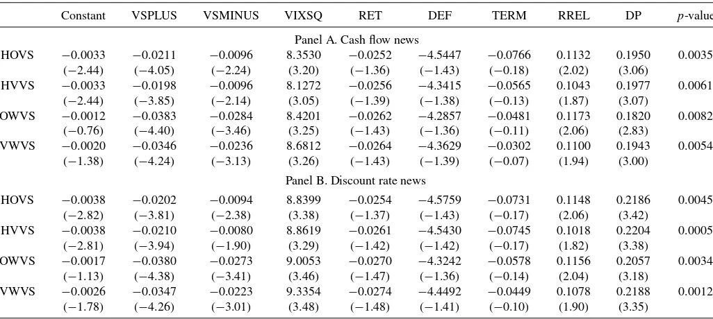
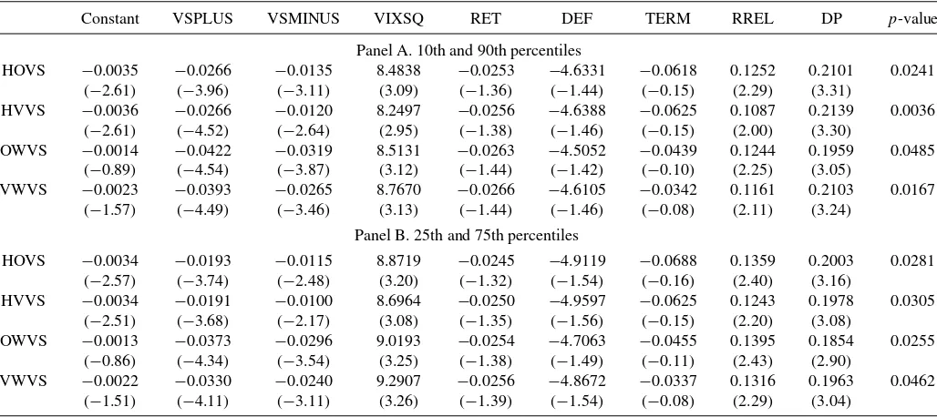
After decomposing aggregate stock returns into one-period expected returns, cash flow news and expected return news, we test whether days associated with extreme news in cash flows and/or expected returns drive the significant negative link between future index returns and implied volatility spreads. If informed investors trade in the options market based on their information about future cash flow and expected return news, we would expect the intertemporal relation between volatility spreads and aggregate returns to be stronger when the magnitude of the unexpected cash flow and/or expected return news is larger. To test this conjecture, we define dummy variables equal to one if the daily cash flow or expected return news are less than the 25th percentile or greater than the 75th percentile among the observed cash flow and expected return news over the sample period. Then, we estimate the asymmetric regression model in Equation(4). We expectβ1 to be more negative (larger in absolute magnitude) than β2 if the information about future cash flow and expected return news affect informed investors’ trades in the options market.
Panels A and B of Table 8 present results for cash flow and expected return news, respectively. The dependent vari-able in all specifications is the one-day ahead excess market returns. The last column presents thep-values associated with the Wald test of the equality of the coefficients of VSPLUS and VSMINUS. For cash flow news, we find that the coefficient of VSPLUS is more negative than the coefficient of VSMINUS for all implied volatility spread measures. For example, the