IPA12-E-122
PROCEEDING, INDONESIAN PETROLEUM ASSOCIATION Thirty-Six Annual Convention and Exhibition, May 2012
THE EFFECT OF RESERVOIR HETEROGENEITY TO DETERMINE THE PATTERN OF WATER INJECTION AND PRODUCTION PILOT
Rudi Kurniawan * HariyadI * Ir. Joko pamungkas *
John H. Simamora**
ABSTRACT
Reservoir Z-600 is one of the oil and gas reservoir located in areas of Pertamina EP WKP Northern Sumatra Region that will be developed into full-scale waterflooding, so it was needed to do a pilot injection to estimate the performance of water injection in each pattern and magnitude of planned water injection which is required for pattern so as to obtaine the optimum amount of oil that can be produced as an overview of the implementation in the field.
The Election candidate workover, injection and production wells is obtained by analysis of scatter plot, bubble map, supported by well history data and overlay permeability distribution map, porosity and oil saturation and the final production of wells. The candidate of pattern is based on the condition of the existing wells, distribution of high porosity and permeability and water cut. It also considers the distance between the wells in a pattern that aims to make time breakthrough does not happen too quickly or too – latter and the properties of rocks between production and injection wells by calculating the heterogeneity in the vertical plane using the method of Dykstra Parson and the driving mechanism acting on the reservoir. The goal is to see the effects of heterogeneity on the pitting of a pilot project in order to obtain maximum displacement efficiency and the effectiveness of optimum water injection rate to acquisition of recovery factor.
The results of the injection rate sensitivity of each pattern to obtain the optimum recovery are pattern peripheral in the compartment A1 with rate of 800 bbl/day obtained cumulative production 5.19
* UPN “Veteran” Yogyakarta ** Pertamina EP -EOR
MMbbl by RF 32.95%. Inverted five spot pattern in the compartment B with rate of 600 bbl/day obtained cumulative production at 3.41 MMbbl with RF 43.56%, and pattern five spot normal in the compartment C2 with rate of 400 bbl/day obtained cumulative production 3.31 MMbbl with RF 31.71%. Pattern five spot inverted obtained the biggest incremental than the other pattern achieve 8.54 % because of the CPV value relative homogeneous and also the distance between wells in this pattern is not too far with time breakthrough average about 8 month with the geological structure of the anticline bounded on the north and south sides of a fault that is leaking. (Please review)
Keywords : Pilot water injection, Pattern, CPV, Scatter Plot, Overlay Map, Reservoir simulation, Rate sensitivity, Recovery Factor
INTRODUCTION
Reservoir Z-600 is one of the reservoir with oil and gas located in the area WKP Pertamina EP Northern Sumatra region which is located approximately 110 km northwest of Medan and 45 km northwest next to Pangkalan brandan. Regionally, reservoir “A” is located in the central part of north Sumatra basin and bounded by the arc asahan in the south and bordered by a series of bukit barisan. – Please review.
The study area of this basin is one of the -three arc basin behind “back arc” which is adjacent to the northeast Bukit barisan, Sumatra. The boundaries of the North Sumatra Basin and regional tectonic el ements that are found showing the - location of the study area within the framework of Tectonic Map of North Sumatra Basin formed in the Late Paleogene and physiographic located between the exposure of Malacca to the east and west of Bukit barisan.
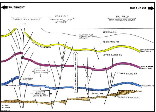
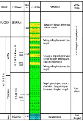
General description of stratigrahpy of north Sumatra which is sedimentation began with deposition of coarseclastikafrom Parapat Formation in Oligocene times. The lower part was deposited in fluvial environment and in some places slowly transformed into a shallow marine environment. Aligned on top, black shale deposited from Bampo closed envir onment ("euxinic"). In the early of Miocene, the shallow marine basin was opened. Belumai formations consisting of domination limes tone deposited at this time.
Reservoir Z-600 has content of initial oil in place (OOIP) 129.3 MMBBL with cumulative production (up to februari 2011) 35 MMBBL and recovery factor among 27%. Drive mechanism acting in this reservoir are combination between water drive and solution drive. This reservoir will be developed into full-scale waterflooding so it was needed to do a pilot project that will be implemented by pheriperal injection pattern, normal and inverted five spot base on scatter plot analysis, status of wells, well history, overlay maps porosity, permeability and oil saturation and also consider about distance and reservoir heterogeneity between the candidate of well production and well injection which is planned with perform sensitivity of the water injection rate, and also candidate of well workover which aimed to improve oil recovery factor.
METHOD
Preparation and Processing of Data
Preparation and processing data is the first and the most important step to do in reservoir simulation, the process begin with collecting required data, classification and selection of field data. Most of these data cannot be directly used, but required processing data to produce a ready use. Form of inputing data to a simulator usually such as a polynomial representation or tabulation (table look-up). Polynomial form mainly used for fluid data and PVT as well as some correlation data. Inputing data in table look-up are more common and easy to use, because some of PVT data are not easily represented graphically.
Geological Data
Geological data which was used to construct the reservoir model include contour structure map, isopach map, isoporosity map, isopermeability map, relperm map, isosaturation map. Those map are
made based on seismic data, drilling cutting, coring and logging.
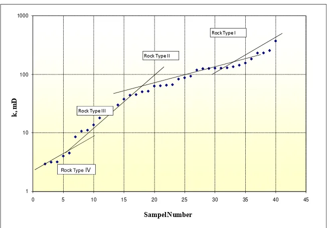
Determination of Rock Region
Rock Region in simulation model are required by simulator to determine the movement fluid flow within the cell and directly related with reservoir characteristics that are to split/ separate/ classify the property which is bad or good. In this paper by classifying permeability based on reservoir characteristic which is then applied to a 3D model.
Processing of Data SCAL
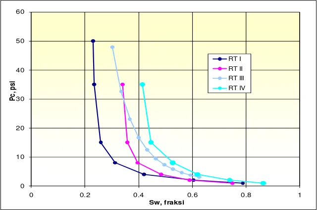
SCAL data which is required in reservoir simulation are rock compressibility, kro;krw vs Sw, krg;krovs Sw and Pc vs Sw.. SCAL data was obtained from samples of core, before it was used as an input to simulation, the data should be processed first to obtain a representative scal data. Processing of relative permeability data from core samples made with Normalization and Denormalization method. Further, the result of this processing are used as input data for relative permeability in simulator, processing of capillary pressure data from core samples conducted by Leverett J-Function method.
Fluid Reservoir Data
Physical properties of reservoir fluid have to be evaluated for reservoir simulation, the physical properties include Bo, Bg, Bw, o, g, w, Rs. The data above can be obtained from the measurement in the laboratory, if the data isn’t available can be calculated by using standart correlation such as Standing, Frik, Glaso, Lasater, Carr Kobayasshi-Burrows. The selection of this correlation is adapted by the field condition.
Production Data
Bubble map Analysis
Bubble Map analysis performed to determine the drainage area of fluid in productive layer. Based on drainage area from bubble map area of oil distributionl, water and gas can be determined to develop strategy of production layer on the object of field.
Pressure Data
Pressure data are obtained from analysis of pressure test (PBU and PDD). Pressure analysis in a field carried out every six month and while it has produced long enough usually done in annual basis. Pressure test performed at a certain depth of the reservoir with reference to date, month and year of measurement.
Flow Rate Data
Flow rate data is required by simulator to calculate the production capacity at a well in a system. These data include productivity index, injectivity index, optimum flow rate and maximum allowable drawdowns. In addition to the data mentioned, there are also other data required in simulation which are mechanical data including, casing size, tubing size, and removal capacity/lift capacity. Economic data including: $/bbl, $/well, economic limit.
Supporting data include: skin, fracture, workover, well history, depth of interval perforation, start of production wells and the end of forecast.
Scatter Plot Analysis
Scatter Plot Analysis shows the wells that have high water cut on the cumulative production which have been achieved for the reservoir. Based on the number of water cut each analysis of wells, it can classify by the wells which have high water produce, medium water produce and low water produce. This analysis also gives an overview in general as a candidate of well production and well injection based on the cumulative water cut.
Calculation Method of Reservoir Heterogeneity by Dykstra Parson Permeability Variation
Reservoir heterogeneity is defined as variation of reservoir properties a the function of areal, ideally when the reservoir is homogeneous then the calculation of reservoir properties in one place will define the state of whole reservoir, however, if
reservoir is heterogeneous we need to predict the variation of reservoir properties as the function of location such as permeability, porosity, saturation, thickness and depositional environment. Dykstra parson introduced the concept of coefficient permeability variation as statistic to calculate inequality data which applies to the permeability variation and it could be to the other rock properties.
Water Injection as Secondary Recovery
In the secondary recovery, injection is performed in order to acquire the remaining reserve in the reservoir that can not be taken in the primary recovery. In such an operation, a fluid is injected into the reservoir not only to maintain the energy of reservoir but also to displace the remaining oil from the reservoir. Injection is done by “dispersed water injection” where water is injected into the oil zone in the lateral direction to the production well according with the pattern of injection. In general, existing producing wells – prior to being converted to injection.. If a new well is needed it is necessary to determine where to place of new well. In areas where the rest of oil is still high probably need more production wells tin thatarea. Isopermeability map also helps in choosing the direction of flow so that the penetration of fluid injection (breakthrough) do not occur prematurely.
One way to improve the oil recovery is to create a pattern of production – injection well with the principle that the existing wells should be used as full as possible during the time of injection. In this paper the pattern which used are peripheral and five spot as a pilot project that aim to try to apply to the problem in the field which this pattern is more often used in waterflooding.
Location and Spread of Injection Well
Consideration in determining the pattern on injection depends on the uniformity of formation include spread toward lateral and vertical permeability, structure of reservoir rock including faulting, slope, topography and economics.
Determination of Well Injection Pattern
central, peripheral edge flooding and pattern flooding.
Depth of Injection Well
Factors that determine the depth of injection is the depth of the reservoir and where the interval selected by the injection.the depth of injection need to know let the injection can be directed precisely to the reservoir.
Determination of Pressure and Injection Rate Achieving the maximum of economic benefit usually an optimal flow injection is injected. Lower limit of rate is rate which can produce oil in its economic limit, while the upper limit of rate is the rate associated with the pressure injection which occur reservoir fracture.
Reservoir Simulation
Definition of Reservoir Simulation
Reservoir simulation is defined as the utilization of artificial model that describe the actual behavior, so it can be used to learn, know and predictthe performance of fluid flow in reservoir system. The selection of the reservoir simulation model based on the needs of desired result as the output, because the proper use will make simulation perform effectively and efficiently. In its development, reservoir simulation divide into three types :
a. Black Oil Simulation
Type of this reservoir is used for isothermal condition, the simultaneous flow of oil, gas and water related to the viscosity, gravity and capillary forces. Black oil used to indicate that type of homogeneous fluid without considering the chemical composition although gas solubility in oil and water are calculated.
b. Thermal Simulation
This simulation is widely used to study of fluid flow, heat transfer and chemical reaction. Thermal simulation is widely used for study of steam injection and oil recovery in the advance stage (insitu combustion)
c. Compositional Simulation
This simulation is used if the composition of the liquid or gas calculated to change in pressure. Usually used to study behavoiur of
the reservoir which containing the volatile-oil and gas condensate.
The Execitution Steps of Reservoir Simulation Basically the steps of work in reservoir simulation include :
1. Preparation Data 2. Modelling 3. Input data,
4. Validation data (inisialisasi data) 5. Prediction and analysis
Preparation Data
Preparation data aims to obtain valid data, and as needed based on the objectives and proprieties of the simulation.. Data needed to perform the simulation can be obtained from various source of data which are possible.Data may require to be processed before being used.. The selection of data sources and processing also affects the readiness of the data itself, which in turn also affects the simulation result as a whole.
Input Data
The process of inputing data into the simulator can be done in three ways that are typing, by typing the data into available colomn. Digitizing is the process of recording the coordinates x and y from existing geological map as much as possible in order to establish the boundary line of good map. Importing is put in a file that is set from another program, so it will be easier in attempt of inputting data, the data entry can be processed by another program in accordance with the format of the input data to the simulator and upon simulation can e taken at once without having to fill one by one.
Initialization
The output from initialization can be compared with the calculated initial oil in place as conventional in order to know the truth of initialization process. Repetition of initialization process is done by adjusting the parameter of physical properties of rock which affects the amount of OOIP such as Net to Gross (NTG), porosity (Ø) and capilary pressure (Pc), oil formation factor, depth of WOC and GOC. Adjusment of initial reservoir pressure is done by changing tne number of certain depth, parameter which is modified for initial pressure initialization in the datum depth.
The goal to be achieved at this stage is to align the initial condition of reservoir model with actual reservoir condition. Initialization process is said have been reached if the initial pressure and OOIP from simulation have been aligned (the difference between actual and simulation result with <1%, the initialization process is considered completed and the simulation process can proceed to the next stage.
History Matching
History matching is the process of modifying the parameter which used in model building in order to create alignment between model and actual condition,
which are based on measured parameter data over a period of time. At this stage the alignment done between production rate and pressure between the calculation result base simulator base on the inputting data with the production data and actual pressure, the alignment is shown by graph of pressure versus time and production of the time.. history matching can be divided into :
Alignment of the production rate
Simulator will calculate flow rate after the number of the real pressure inserted. This alignment is done when oil rate graph obtained do not correspond to the actual flow rate, this process done by changing the relative permeability until its reached the alignment of simulation model with the real model.
Alignment of Pressure
Alignment of Pressure can be done by modifying the size of aquifer, rock compressibility, transmisibilities
kh
and skin factor. The sizeof aquifer will be related to the energy that will push oil into the wellbore, by changing the size of
aquifer so pressure in the reservoir system will change as well as alteration of compressibility rock data and trasmisibility will influence the size of number of pressure in the reservoir.
Quality of history matching and trustworthiness of the model depend on the number of historical production data which is available to be harmonized. History matching can be done with the description of different reservoir, when the data are incompleteAlignment fails ,when the available data indicates that a number of assumption in the development model must be repaired. This assumstion include geological structures, PVT behavior, reservoir area and presence of aquifer. The failed alignment for some case indicate that there are inaccuracies of available data.
The accuracy of prediction of reservoir performance for the future depend on the amount of available data for history matching, reservoir performance prediction accuracy will decrease with increasing time, for that it is necessary for updating reservoir simulation study. Updating is done after a period of time to align the production to align the new production historical data.
Prediction
Prediction or forecasting is the final step in reservoir simulation. This stage aims to find out or to know the behavior of reservoir which simulated to the future based on expected condition.
Reservoir model that have been aligned with the actual condition of reservoir can be used for forecasting of reservoir bahaviour for production scenario which can be applied to the actual reservoir in the field. Determination through from the forecasting model is strongly influenced by the quality of the resulting alignment and the quality of alignment was influenced by the amount of mass production basis and how to modify the physical properties of reservoir rock and fluid to get the alignment.
RESULT
about 223 wells by the number of active wells until now about 15 wells with 8 active producing oil and 7 active injection wells. Last oil producing in this reservoir in february 2012 for 296 bbl/d with water cut 54%.
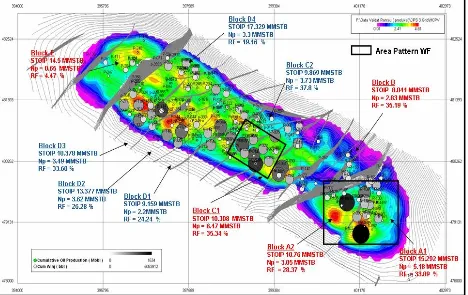
In december 2010 conducted pilot water injection with periheral pattern in compartment A1 with 2 injection wells and 2 production wells, which the result is not effective to push oil, because of the distance between injection and production well are far enough with the injection rate is not optimal to displace oil with oil recovery obtained until february 2036?? with cumulative production among 4.75 MMBBL. Last cumulative production in compartment A1 among 4.6 MMBBL.with recovery factor of 30.24% obtained incremental recovery from February 2011 until February 2036 amount 1.02% , so that based on that incremental it is necessary to repair the injection pattern and optimum rate injection to increase the effectiveness of sweep and oil recovery. A large number of oil can be taken underlies need to further study the filed development in order to enhance oil recovery in reservior Z-600.
Reservoir Simulation
Proces of simulation in reservoir Z-600 field Rantau begins with the following stage : preparation data include of geological data, data scal, fluid and production data, completion, modeling and grid, initialization, histort matching and prediction. Relative permeability data in reservoir Z-600 obtained from SCAL result from laboratory. Krw and Kro are function of Sw resulf of averaging core samples to obtain the representative relative permeability in reservoir Z-600 from core samples well P-377 and P-398 by
Normalization – Denormalization method that can be seen in Appendix B. Capillary pressure data for input data obtained from core sample well P-377, to get the represent Pc in reservoir Z-600 made by method averaging Laverett J-Function which can be seen in appendix B. for PVT data obtained through the analysis of PVT in laboratory.
After preparation data, then input data. This process done after all the necessary data collected, the data include geological data, physical properties of rock, physical properties of fluid and other supporting data such as historical data production, pressure and well perforation. The process of inputing data into simulator aims to build a reservoir model. Character modeling is shown in Table 3. Making grid which
too much will result in a more rigorous simulation calculation, but more time needed by simulator to perform the calculation.
Once the input data was obtained then the process to reservoir model initialization, this process aims to equalize the initial reservoir pressure and original oil in place simulation result with actual condition. Initialization process reservoir Z-600 has been done well, it is seen from the small difference in actual and simulation result OOIP of 0.48% and the difference initial pressure between actual and simulation result of 0.014%.
The next stage is alignment (history matching), this stage aims to align the model which has been built with the actual condition based on measured parameter during the period of time, parameter that aligned are fluid production rate (oil, water, gas) and also reservoir pressure. History matching in reservoir Z-600 focused in the compartment which have the biggest cumulative production, this is because of the reconstruction production data from 1930 until 1968 result of missing record data, and the invalid record of production data water and gas.. The result of history matching can be seen in Appendix D.
Once the alignment has been done, next to Productivity Index Matching (PI Matching) during the last six month before the end of history matching and six month after the end of history matching. PI matching done to align the productivity of reservoir model with actual reservoir let the perform of model actually resembles the actual reservoir performance. The parameter was changed during PI matching are data skin, productivity index, table vertical flow performance. Prediction is the final step to conducting reservoir simulation after the process of history matching and PI matching. This stage aims to find out the behavior of simulated reservoir at the future time under the expected condition, prediction made during 25 years up to February 2036 with several alternative development scenario in an effort to improve oil recovery. Scenario consist of three scenarios, namely :
Scenario I (BC) : 8 production wells dan 7 injection wells existing
Scenario II : Skenario I + 19 well Workover
Scenario I predicted for 25 years (March 2012 - February 2036) based on existing wells, 8 production wells (361, R-032HZ, 391,022, P-383, P-335, P-346, P-106) and 7 injection wells (P403-iw, R153-iw, R107-iw, P025-iw, P239-iw, P377-iw, P309-iw). Based on scenario I obtained cumulative oil production of 35.65 MMSTB and recovery factorof 27.58%.
Scenario II is scenario I added 19 wells workover monitor. Based on scenario II obtained cumulative oil production of 40.863 MMSTB and recovery factorof 31.61%.
Scenario III is scenario II plus water injection with pattern peripheral, inverted five spot and normal five spot as pilot project with the intention of compartment A1, B and C2 which aims to see the reservoir behaviour about there is water influx from outside into cumulative production and recovery factorthat is produced as a reference that is used later when the reservoir developed into a full scale waterflood. The result obtained were compared with a sensitivity rate of water injection that aims to determine tie optimal injection rate based on the type of pattern used.
Peripheral pattern based on the sensitivity of water injection rate obtained optimum injection rate which give the greatest cumulative oil production of 800 bbl/day where there are 4 injection wells (P402-iw, P403-iw, P404-iw dan R153-iw), the distance between well production – injection on this pattern ranged from 285 – 666 m, with average permeability each wells range 83- 118 md obtained break trough time for 5 – 7 month. Break trough time obtained based on increase of water production rate and water cut after 5 month injection and decrease of oil production rate and oil cut plot after some period time which are shown in the oil production well P361 and R032-HZ which can be seen in Table 6.
Five spot normal pattern, based on the sensitivity of water injection rate obtained optimum injection rate which give the greatest cumulative oil production of 400 bbl/day. the distance between well production – injection on this pattern ranged from 129 – 480 m, with average permeability each wells range 5- 138 md obtained break trough time for 12 month. Break trough time obtained based on increase of water production rate and water cut after 12 month injection and decrease of oil production rate and oil cut plot after some period time which are shown in
the oil production well P168 which can be seen in Table 6.
five spot inverted pattern, based on the sensitivity of water injection rate obtained optimum injection rate which give the greatest cumulative oil production of 600 bbl/day, with 1 well injection and 4 well production obtained time break trough which vary from each well production, it can be seen from average permeability each well that vary each and other supported by the distance between production and injection wells. Time break trough from this pattern can be seen in Table 6. Pattern five spot inverted obtained the biggest incremental than the other pattern achieve 8.54 % because of the CPV value relative homogeneous and also the distance between wells in this pattern is not too far with time breakthrough average about 8 month with the geological structure of the anticline bounded on the north and south sides of a fault that is leaking.
based on the result of water injection sensitivity obtained that the pattern of peripheral with optimum rate of 800 bbl/day, pattern of five spot inverted with optimum rate of 600 bbl/day, pattern of five spot normal with optimum rate of 400 bbl/day, implemented as scenario III with cumulative oil production of 41.91 MMBBL and recovery factor 32.42% giving the greatest recovery factor by giving the highest cumulative oil production average from each well. So that the scenario III is recommended as reservoir development scenario in reservoir “A” as the implemented of pilot project.
CONCLUSION
Based on the result of reservoir simulation in reservoir Z-600, then it can be concluded as follow :
1. Initialization phase include initial pressure and OOIP between reservoir model and actual condition have been successfully performed, it is seen from the difference between pressure model and actual of 0.014% and OOIP between reservoir model and actual of 0.48%.
3. Based on the planned scenario, obtained that scenario III is the best scenario with the implementation of pilot injection by peripheral with 800 bbl/d water injection, five spot normal with 400 bbl/d water injection, five spot inverted with 600 bbl/d water injection produce cumulative oil production of 41.823 MMBBL and recovery factor 32.42% and incremental recovery factor from base case of 4.84%.
REFERENCE
Ahmed, Tarek., 2000, Reservoir Engineering Handbook, Gulf Publishing Company, Houston, Texas,.
Amyx, J.W., Bass, D.W.Jr., Whiting, R.L, 1660, Petroleum Reservoir Engineering Physical Properties, Mc Graw Hill Books Company, New York, Toronto, London.
Aziz, K. And Settari, A., 1979, Petroleum Reservoir Simulation, Elsevier Applied Science Pubisher, London and New York.
Crichlow, H.B., 1997, Modern Reservoir Engineering A Simulation Approach. Prentince Hall, Inc., Englewood Cliffs, New Jersey.
Willhite, G. Paul, 1986Waterflooding, Third Printing, Society of Petroleum Engineer, Richardson, Texas.
Forrest F. Craig, Jr., 1971, The Reservoir Engineering Aspects of Waterflooding, SPE Monographs Vol.3, Dallas.
Tim LPPM UPN “Veteran” Yogyakarta, Studi Plan of Further Development (POFD) Waterflood Full Scale, RANTAU FIELD, PERTAMINA EP”, Yogyakarta, 2011.
Rukmana, Dadang. Sutadiwiria, Gunawan., Bahan Acuan Studi Reservoir Simulasi dan Decline Analysis, Divisi kajian dan Pengembangan. BP MIGAS.
ACKNOWLEDGEMENTS
Rock Type I
k >232.7 md
Rock Type II
44 < k < 184
Rock Type III
37.70 < k < 8.5
Rock Type IV
k < 8.5 md
TABLE 1 - DISTRIBUTION OF ROCK TYPE ( see Figure 16 )
Rock Type Sumur Sampel Ka Porosity Swc Kro@Swc Krw@Sor Sor Number mD fraksi fraksi fraksi fraksi fraksi I P-377 16 128 0.2618 0.2229 0.0527 0.040397 0.4888 II P-398 1E 50.49 0.2082 0.4371 0.164448 0.029778 0.31418
7E 83.39 0.2951 0.4219 0.074397 0.16479 0.34044 III P-377 14 30 0.245 0.2946 0.0521 0.034227 0.3972
13 27 0.2449 0.3099 0.0983 0.030254 0.3533 IV P-377 17 18 0.2381 0.3601 0.0917 0.065405 0.3046 TABLE 2 - WATER – OIL RELATIVE PERMEABILITY DATA ( see Figure 17 )
Uraian Reservoir “A”
Jenis Grid Cartesian
Jumlah Grid 112 x178 x 22 = 438592 grid
Total Jumlah Grid 438592
Grid Aktif 196310
Sistem Porositas Dual Porosity
Jumlah sektor 11 sektor
WOC 670 m = 2198.163 ft
Tekanan Awal 1243 psia
Mekanisme Pendorong Kombinasi Water Drive dan Solution Drive
Datum 670 m
PVT 1
Simulator Black Oil (IMEX)
AKTUAL SIMULASI PERBEDAAN
MMBBL
MMBBL
%
CUM LIQUID
53.9
53.84
0.11
CUM OIL
35.06
35.01
0.13
CUM WATER
18.84
17.82
5.4
DATA
TABLE 4 - INITIALIZATION RESULT RESERVOIR Z-600
TABLE 5 - HISTORY MATCHING RESULT
TABLE 6 - ANALYSIS OF PILOT PROJECT
WELL
STATUS
Pattern RATE
OPTIMUM Distance
(M)
CPV
K
avg
TIME
BREAKTROUGH
P168
PROD
WELL
0
0.1925
137.95
P307
‐
IW
480.89
0.9077
82.2
P310
‐
IW
341.47
0.5163
51.75
P338
‐
IW
300.87
0.139
87.45
P347
‐
IW
129.7
0.43
72.5
P252
448.31
0.356
56
7
MONTH
R053
416.25
0.631
61.3
5
MONTH
R110
506.21
0.521
53.4
6
MONTH
R114
405.5
0.365
70
8
MONTH
R129
‐
IW
INJ
WELL
0
0.187
85.6
‐
P361
0
0.462
186
5
MONTH
R032
‐
HZ
285.7
0.265
83.54
7
MONTH
P402
‐
IW
422.28
0.503
117.31
‐
P403
‐
IW
665.12
0.187
98.6
‐
P404
‐
IW
362.3
0.356
85.87
‐
R153
‐
IW
494.23
0.537
92.4
‐
12
MONTH
IN
J
WELL
PR
O
D
WELL
PROD
WELL
OOIP NP @ 2011 RF @ 2011 NP @ 2035 (SIMULASI) RF ΔRF
MMSTB MMSTB % MMSTB % %
SKENARIO 1 (BC) 35.64 27.67
-SKENARIO 2 (BC + WO) 40.86 31.61 4.03
SKENARIO 3 (BC + WO + INJ) 41.91 32.42 4.84
129.268 35.007 27.08 SKENARIO
OOIP NP @FEB 2011 NP @ FEB 2036
MMBBL MMBBL MMBBL
PERIPHERAL @ 2010 A1 15.742 4.6 29.22 4.76 30.23 1.01 PERIPHERAL @ 2013 A1 15.742 4.6 29.22 5.19 32.95 3.73
FIVE SPOT INVERTED B 7.835 2.74 34.97 3.41 43.56 8.59
FIVE SPOT NORMAL C2 10.45 3.11 29.76 3.31 31.71 1.95
RF
RF @ FEB 2011 RF @ FEB 2036
BLOK POLA INJEKSI
TABLE 7 - RESULT OF RF DEVELOPMENT SCENARIO
APPENDIX A (Geological Finding and Reviewing)
Figure 1 - Location of Reservoir Z-600
Paleogen
Neogene
Paleocene
Eocene
Oligocen
Miocene
P lei s toc en Pl io c e n Qu a rt e rn a ry
GEOLOGICAL
TIME SCALE
SOURCE ROCK
RESERVOIR ROCK
SEAL ROCK
TRAP FORMATION
GENERATION
SOURCE ROCK
MATURITY
MIGRATION/
PRESERVATION
CRITICAL MOMENT
L
U
L
U
L
M
U
L
M
U
Bruksah
Belumai P eut u Baong L o w e r K e u ta p a n gBampo
Structural Rift RelatedBampo
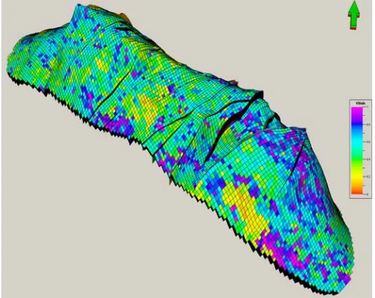
Belumai Baong Structural Stratigraphic Baong Structural Stratigraphic Structural Stratigraphic Se u ru laFigure 6 - Final 3D Structure Model Figure 5 - Compartment Spreading in Field Rantau
Figure 8 -3D V-Shale Model
APPENDIX B (Preparation Data)
Figure 10 - Grid Top Map
Figure 12 - Net to Gross Map
Figure 13 - Isoporosity Map
1 10 100 1000
0 5 10 15 20 25 30 35 40 45
k,
m
D
Sampel Number
Rock Type I
Rock Type II
Rock Type III
0 0.02 0.04 0.06 0.08 0.1 0.12 0 0.02 0.04 0.06 0.08 0.1 0.12
0 0.1 0.2 0.3 0.4 0.5 0.6 0.7 0.8 0.9 1
K rw , f ra ksi K ro , f ra ksi Sw, fraksi
RT Kro I RT Kro II RT Kro III RT Kro IV RT Krw I RT Krw II RT Krw III RT Krw IV
Figure 17 - Plot Rock Type Water – Oil Relative Permeability
0 10 20 30 40 50 60
0 0.2 0.4 0.6 0.8 1
Pc , p si Sw, fraksi RT I RT II RT III RT IV
.
0 20 40 60 80 100 120 140
0 500 1000 1500 2000 2500
Rs
,
V/V
Tekanan, Psig
0 0.1 0.2 0.3 0.4 0.5 0.6
0 200 400 600 800 1000 1200
Bg
Tekanan, Psig
Figure 19. Plot Pressure vs Rs
Figure 21 - Plot Pressure vs Bg
1 1.05 1.1 1.15 1.2 1.25 1.3
0 500 1000 1500 2000 2500
Bo
(v/
V
)
Tekanan, Psig
APPENDIX C (Pilot Injection Pattern)
Figure 24 - Bubble Map Cum Oil vs Net Pay
Figure 26 - Bubble Map Cum Oil vs Permebility
Figure 28 - Scatter Plot Analysis zone Z-600 field Rantau
Figure 30 - Five Spot Inverte Pattern Compartment B
Figure 32 - History Matching Of Pressure
Figure 34 - History Matching of Oil Rate
Figure 36 - Sensitivity Rate Injection Peripheral
5.1858 5.186 5.1862 5.1864 5.1866 5.1868 5.187
0 200 400 600 800
Cu
m
O
il,
MMB
bl
Rate
Inj,
Bbl/D
Figure 37 - Sensitivity Rate Injection Five Spot Normal
3.1175 3.118 3.1185 3.119 3.1195 3.12
0 200 400 600 800
Cu
m
O
il,
MMB
b
l
4.14 4.17 4.2 4.23 4.26 4.29 4.32 4.35 4.38 4.41
0 200 400 600 800
Cu
m
Oi
l,
MMB
b
l
Rate
Inj,
Bbl/D
Figure 38 - Sensitivity Rate Injection Five Spot Inverted