OpenCL
Programming Guide
T
he OpenGL graphics system is a software interface to graphics hardware. (“GL” stands for “Graphics Library.”) It allows you to create interactive programs that produce color images of moving, three-dimensional objects. With OpenGL, you can control computer-graphics technology to produce realistic pictures, or ones that depart from reality in imaginative ways.The OpenGL Series from Addison-Wesley Professional comprises tutorial and reference books that help programmers gain a practical understanding of OpenGL standards, along with the insight needed to unlock OpenGL’s full potential.
Visit informit.com /opengl for a complete list of available products
OpenGL
®OpenCL
Programming Guide
Aaftab Munshi
Benedict R. Gaster
Timothy G. Mattson
James Fung
Dan Ginsburg
Upper Saddle River, NJ • Boston • Indianapolis • San Francisco
New York • Toronto • Montreal • London • Munich • Paris • Madrid Capetown • Sydney • Tokyo • Singapore • Mexico City
Many of the designations used by manufacturers and sellers to distin-guish their products are claimed as trademarks. Where those designa-tions appear in this book, and the publisher was aware of a trademark claim, the designations have been printed with initial capital letters or in all capitals.
The authors and publisher have taken care in the preparation of this book, but make no expressed or implied warranty of any kind and assume no responsibility for errors or omissions. No liability is assumed for incidental or consequential damages in connection with or arising out of the use of the information or programs contained herein.
The publisher offers excellent discounts on this book when ordered in quantity for bulk purchases or special sales, which may include elec-tronic versions and/or custom covers and content particular to your business, training goals, marketing focus, and branding interests. For more information, please contact:
U.S. Corporate and Government Sales (800) 382-3419
For sales outside the United States please contact: International Sales
[email protected] Visit us on the Web: informit.com/aw
Cataloging-in-publication data is on file with the Library of Congress.
Copyright © 2012 Pearson Education, Inc.
All rights reserved. Printed in the United States of America. This pub-lication is protected by copyright, and permission must be obtained from the publisher prior to any prohibited reproduction, storage in a retrieval system, or transmission in any form or by any means, elec-tronic, mechanical, photocopying, recording, or likewise. For informa-tion regarding permissions, write to:
v
Contents
Figures . . . xv
Tables . . . .xxi
Listings . . . xxv
Foreword. . . .xxix
Preface . . . .xxxiii
Acknowledgments . . . xli About the Authors . . . xliii
Part I The OpenCL 1.1 Language and API . . . .1
1. An Introduction to OpenCL . . . 3
What Is OpenCL, or . . . Why You Need This Book . . . 3
Our Many-Core Future: Heterogeneous Platforms . . . 4
Software in a Many-Core World . . . 7
Conceptual Foundations of OpenCL . . . 11
Platform Model . . . 12
Execution Model . . . 13
Memory Model . . . 21
Programming Models . . . 24
OpenCL and Graphics . . . 29
The Contents of OpenCL . . . 30
Platform API . . . 31
Runtime API . . . 31
Kernel Programming Language . . . 32
OpenCL Summary. . . 34
The Embedded Profile . . . 35
2. HelloWorld: An OpenCL Example . . . 39
Building the Examples. . . 40
Prerequisites. . . 40
Mac OS X and Code::Blocks . . . 41
Microsoft Windows and Visual Studio . . . 42
Linux and Eclipse . . . 44
HelloWorld Example . . . 45
Choosing an OpenCL Platform and Creating a Context . . . 49
Choosing a Device and Creating a Command-Queue . . . 50
Creating and Building a Program Object . . . 52
Creating Kernel and Memory Objects . . . 54
Executing a Kernel . . . 55
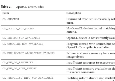
Checking for Errors in OpenCL . . . 57
3. Platforms, Contexts, and Devices . . . 63
OpenCL Platforms . . . 63
OpenCL Devices . . . 68
OpenCL Contexts . . . 83
4. Programming with OpenCL C . . . 97
Writing a Data-Parallel Kernel Using OpenCL C . . . 97
Scalar Data Types . . . 99
The half Data Type . . . 101
Vector Data Types . . . 102
Vector Literals . . . 104
Vector Components. . . 106
Other Data Types . . . 108
Derived Types . . . 109
Implicit Type Conversions. . . 110
Usual Arithmetic Conversions . . . 114
Explicit Casts . . . 116
Explicit Conversions . . . 117
Reinterpreting Data as Another Type . . . 121
Vector Operators . . . 123
Arithmetic Operators . . . 124
Contents vii
Bitwise Operators . . . 127
Logical Operators . . . 128
Conditional Operator . . . 129
Shift Operators . . . 129
Unary Operators . . . 131
Assignment Operator . . . 132
Qualifiers . . . 133
Function Qualifiers . . . 133
Kernel Attribute Qualifiers . . . 134
Address Space Qualifiers . . . 135
Access Qualifiers . . . 140
Type Qualifiers . . . 141
Keywords . . . 141
Preprocessor Directives and Macros . . . 141
Pragma Directives . . . 143
Macros . . . 145
Restrictions . . . 146
5. OpenCL C Built-In Functions . . . 149
Work-Item Functions. . . 150
Math Functions . . . 153
Floating-Point Pragmas . . . 162
Floating-Point Constants . . . 162
Relative Error as ulps . . . 163
Integer Functions. . . 168
Common Functions . . . 172
Geometric Functions . . . 175
Relational Functions . . . 175
Vector Data Load and Store Functions . . . 181
Synchronization Functions . . . 190
Async Copy and Prefetch Functions . . . 191
Atomic Functions . . . 195
Miscellaneous Vector Functions . . . 199
Image Read and Write Functions . . . 201
Reading from an Image . . . 201
Samplers . . . 206
Writing to an Image . . . 210
Querying Image Information . . . 214
6. Programs and Kernels . . . 217
Program and Kernel Object Overview . . . 217
Program Objects . . . 218
Creating and Building Programs . . . 218
Program Build Options . . . 222
Creating Programs from Binaries . . . 227
Managing and Querying Programs . . . 236
Kernel Objects . . . 237
Creating Kernel Objects and Setting Kernel Arguments . . . 237
Thread Safety. . . 241
Managing and Querying Kernels . . . 242
7. Buffers and Sub-Buffers. . . 247
Memory Objects, Buffers, and Sub-Buffers Overview. . . 247
Creating Buffers and Sub-Buffers . . . 249
Querying Buffers and Sub-Buffers. . . 257
Reading, Writing, and Copying Buffers and Sub-Buffers . . . 259
Mapping Buffers and Sub-Buffers . . . 276
8. Images and Samplers . . . 281
Image and Sampler Object Overview . . . 281
Creating Image Objects . . . 283
Image Formats . . . 287
Querying for Image Support . . . 291
Creating Sampler Objects . . . 292
OpenCL C Functions for Working with Images . . . 295
Transferring Image Objects . . . 299
9. Events . . . 309
Commands, Queues, and Events Overview . . . 309
Events and Command-Queues . . . 311
Contents ix
Generating Events on the Host . . . 321
Events Impacting Execution on the Host . . . 322
Using Events for Profiling . . . 327
Events Inside Kernels . . . 332
Events from Outside OpenCL . . . 333
10. Interoperability with OpenGL . . . 335
OpenCL/OpenGL Sharing Overview . . . 335
Querying for the OpenGL Sharing Extension . . . 336
Initializing an OpenCL Context for OpenGL Interoperability . . . . 338
Creating OpenCL Buffers from OpenGL Buffers . . . 339
Creating OpenCL Image Objects from OpenGL Textures . . . 344
Querying Information about OpenGL Objects. . . 347
Synchronization between OpenGL and OpenCL . . . 348
11. Interoperability with Direct3D . . . 353
Direct3D/OpenCL Sharing Overview . . . 353
Initializing an OpenCL Context for Direct3D Interoperability . . . . 354
Creating OpenCL Memory Objects from Direct3D Buffers and Textures. . . 357
Acquiring and Releasing Direct3D Objects in OpenCL . . . 361
Processing a Direct3D Texture in OpenCL . . . 363
Processing D3D Vertex Data in OpenCL. . . 366
12. C++ Wrapper API . . . 369
C++ Wrapper API Overview . . . 369
C++ Wrapper API Exceptions . . . 371
Vector Add Example Using the C++ Wrapper API . . . 374
Choosing an OpenCL Platform and Creating a Context . . . 375
Choosing a Device and Creating a Command-Queue . . . 376
Creating and Building a Program Object . . . 377
Creating Kernel and Memory Objects . . . 377
13. OpenCL Embedded Profile . . . 383
OpenCL Profile Overview . . . 383
64-Bit Integers . . . 385
Images . . . 386
Built-In Atomic Functions . . . 387
Mandated Minimum Single-Precision Floating-Point Capabilities. . . 387
Determining the Profile Supported by a Device in an OpenCL C Program . . . 390
Part II OpenCL 1.1 Case Studies . . . 391
14. Image Histogram . . . 393
Computing an Image Histogram . . . 393
Parallelizing the Image Histogram . . . 395
Additional Optimizations to the Parallel Image Histogram . . . 400
Computing Histograms with Half-Float or Float Values for Each Channel . . . 403
15. Sobel Edge Detection Filter . . . 407
What Is a Sobel Edge Detection Filter? . . . 407
Implementing the Sobel Filter as an OpenCL Kernel . . . 407
16. Parallelizing Dijkstra’s Single-Source Shortest-Path Graph Algorithm . . . 411
Graph Data Structures . . . 412
Kernels . . . 414
Leveraging Multiple Compute Devices . . . 417
17. Cloth Simulation in the Bullet Physics SDK . . . 425
An Introduction to Cloth Simulation . . . 425
Simulating the Soft Body . . . 429
Executing the Simulation on the CPU . . . 431
Changes Necessary for Basic GPU Execution . . . 432
Contents xi
Optimizing for SIMD Computation and Local Memory . . . 441
Adding OpenGL Interoperation . . . 446
18. Simulating the Ocean with Fast Fourier Transform . . . 449
An Overview of the Ocean Application . . . 450
Phillips Spectrum Generation . . . 453
An OpenCL Discrete Fourier Transform . . . 457
Determining 2D Decomposition . . . 457
Using Local Memory . . . 459
Determining the Sub-Transform Size . . . 459
Determining the Work-Group Size . . . 460
Obtaining the Twiddle Factors . . . 461
Determining How Much Local Memory Is Needed . . . 462
Avoiding Local Memory Bank Conflicts. . . 463
Using Images . . . 463
A Closer Look at the FFT Kernel . . . 463
A Closer Look at the Transpose Kernel . . . 467
19. Optical Flow . . . 469
Optical Flow Problem Overview . . . 469
Sub-Pixel Accuracy with Hardware Linear Interpolation . . . 480
Application of the Texture Cache . . . 480
Using Local Memory . . . 481
Early Exit and Hardware Scheduling . . . 483
Efficient Visualization with OpenGL Interop . . . 483
Performance. . . 484
20. Using OpenCL with PyOpenCL . . . 487
Introducing PyOpenCL . . . 487
Running the PyImageFilter2D Example . . . 488
PyImageFilter2D Code. . . 488
Context and Command-Queue Creation . . . 492
Loading to an Image Object . . . 493
Creating and Building a Program . . . 494
Setting Kernel Arguments and Executing a Kernel. . . 495
21. Matrix Multiplication with OpenCL. . . 499
The Basic Matrix Multiplication Algorithm . . . 499
A Direct Translation into OpenCL . . . 501
Increasing the Amount of Work per Kernel . . . 506
Optimizing Memory Movement: Local Memory . . . 509
Performance Results and Optimizing the Original CPU Code . . . . 511
22. Sparse Matrix-Vector Multiplication. . . 515
Sparse Matrix-Vector Multiplication (SpMV) Algorithm . . . 515
Description of This Implementation. . . 518
Tiled and Packetized Sparse Matrix Representation . . . 519
Header Structure . . . 522
Tiled and Packetized Sparse Matrix Design Considerations . . . 523
Optional Team Information . . . 524
Tested Hardware Devices and Results . . . 524
Additional Areas of Optimization . . . 538
A. Summary of OpenCL 1.1 . . . 541
The OpenCL Platform Layer . . . 541
Contexts . . . 541
Querying Platform Information and Devices. . . 542
The OpenCL Runtime . . . 543
Command-Queues . . . 543
Buffer Objects . . . 544
Create Buffer Objects. . . 544
Read, Write, and Copy Buffer Objects . . . 544
Map Buffer Objects . . . 545
Manage Buffer Objects . . . 545
Query Buffer Objects. . . 545
Program Objects . . . 546
Create Program Objects. . . 546
Build Program Executable . . . 546
Build Options . . . 546
Query Program Objects. . . 547
Contents xiii
Kernel and Event Objects . . . 547
Create Kernel Objects . . . 547
Kernel Arguments and Object Queries . . . 548
Execute Kernels . . . 548
Event Objects. . . 549
Out-of-Order Execution of Kernels and Memory Object Commands. . . 549
Profiling Operations . . . 549
Flush and Finish . . . 550
Supported Data Types . . . 550
Built-In Scalar Data Types . . . 550
Built-In Vector Data Types . . . 551
Other Built-In Data Types . . . 551
Reserved Data Types . . . 551
Vector Component Addressing . . . 552
Vector Components. . . 552
Vector Addressing Equivalencies. . . 553
Conversions and Type Casting Examples . . . 554
Operators . . . 554
Address Space Qualifiers . . . 554
Function Qualifiers . . . 554
Preprocessor Directives and Macros . . . 555
Specify Type Attributes . . . 555
Math Constants . . . 556
Work-Item Built-In Functions . . . 557
Integer Built-In Functions . . . 557
Common Built-In Functions . . . 559
Math Built-In Functions . . . 560
Geometric Built-In Functions . . . 563
Relational Built-In Functions . . . 564
Vector Data Load/Store Functions. . . 567
Atomic Functions . . . 568
Async Copies and Prefetch Functions. . . 570
Synchronization, Explicit Memory Fence . . . 570
Miscellaneous Vector Built-In Functions . . . 571
Image Objects . . . 573
Create Image Objects. . . 573
Query List of Supported Image Formats . . . 574
Copy between Image, Buffer Objects . . . 574
Map and Unmap Image Objects . . . 574
Read, Write, Copy Image Objects . . . 575
Query Image Objects. . . 575
Image Formats . . . 576
Access Qualifiers . . . 576
Sampler Objects . . . 576
Sampler Declaration Fields . . . 577
OpenCL Device Architecture Diagram . . . 577
OpenCL/OpenGL Sharing APIs. . . 577
CL Buffer Objects > GL Buffer Objects . . . 578
CL Image Objects > GL Textures. . . 578
CL Image Objects > GL Renderbuffers . . . 578
Query Information . . . 578
Share Objects . . . 579
CL Event Objects > GL Sync Objects. . . 579
CL Context > GL Context, Sharegroup. . . 579
OpenCL/Direct3D 10 Sharing APIs . . . 579
xv
Figures
Figure 1.1 The rate at which instructions are retired is the same in these two cases, but the power is much less with two cores running at half the frequency of a
single core. . . .5
Figure 1.2 A plot of peak performance versus power at the thermal design point for three processors produced on a 65nm process technology. Note: This is not to say that one processor is better or worse than the others. The point is that the more specialized the
core, the more power-efficient it is. . . .6
Figure 1.3 Block diagram of a modern desktop PC with multiple CPUs (potentially different) and a GPU, demonstrating that systems today are frequently
heterogeneous . . . .7
Figure 1.4 A simple example of data parallelism where a single task is applied concurrently to each element
of a vector to produce a new vector . . . .9
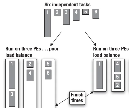
Figure 1.5 Task parallelism showing two ways of mapping six independent tasks onto three PEs. A computation is not done until every task is complete, so the goal should be a well-balanced load, that is, to have the
time spent computing by each PE be the same. . . . 10
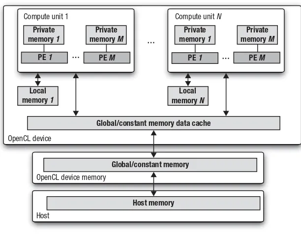
Figure 1.6 The OpenCL platform model with one host and one or more OpenCL devices. Each OpenCL device has one or more compute units, each of which has
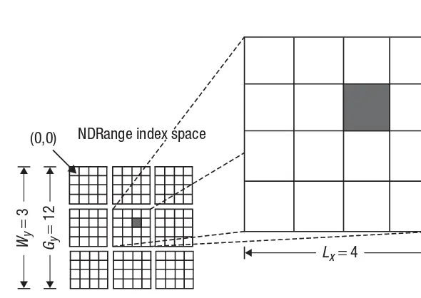
Figure 1.7 An example of how the global IDs, local IDs, and work-group indices are related for a two-dimensional NDRange. Other parameters of the index space are defined in the figure. The shaded block has a global ID of (gx,gy) = (6, 5) and a work-group plus local ID of
(wx,wy) = (1, 1) and (lx,ly) =(2, 1) . . . 16
Figure 1.8 A summary of the memory model in OpenCL and how the different memory regions interact with the platform model . . . .23
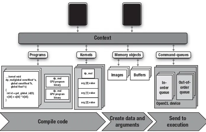
Figure 1.9 This block diagram summarizes the components of OpenCL and the actions that occur on the host during an OpenCL application. . . .35
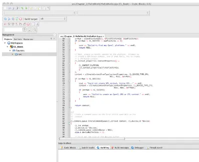
Figure 2.1 CodeBlocks CL_Book project . . . .42
Figure 2.2 Using cmake-gui to generate Visual Studio projects . . . .43
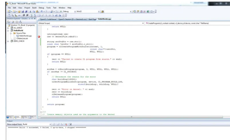
Figure 2.3 Microsoft Visual Studio 2008 Project . . . .44
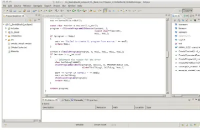
Figure 2.4 Eclipse CL_Book project . . . .45
Figure 3.1 Platform, devices, and contexts . . . .84
Figure 3.2 Convolution of an 8×8 signal with a 3×3 filter, resulting in a 6×6 signal . . . .90
Figure 4.1 Mapping get_global_id to a work-item . . . .98
Figure 4.2 Converting a float4 to a ushort4 with round-to-nearest rounding and saturation . . . .120
Figure 4.3 Adding two vectors . . . .125
Figure 4.4 Multiplying a vector and a scalar with widening . . . .126
Figure 4.5 Multiplying a vector and a scalar with conversion and widening . . . .126
Figure 5.1 Example of the work-item functions . . . 150
Figures xvii
Figure 9.1 A failed attempt to use the clEnqueueBarrier()
command to establish a barrier between two command-queues. This doesn’t work because the barrier command in OpenCL applies only to the
queue within which it is placed. . . 316
Figure 9.2 Creating a barrier between queues using
clEnqueueMarker() to post the barrier in one
queue with its exported event to connect to a
clEnqueueWaitForEvent() function in the other
queue. Because clEnqueueWaitForEvents()
does not imply a barrier, it must be preceded by an
explicit clEnqueueBarrier(). . . 317
Figure 10.1 A program demonstrating OpenCL/OpenGL interop. The positions of the vertices in the sine wave and the background texture color values are computed by kernels in OpenCL and displayed
using Direct3D. . . . .344
Figure 11.1 A program demonstrating OpenCL/D3D interop. The sine positions of the vertices in the sine wave and the texture color values are programmatically set by kernels in OpenCL and displayed using
Direct3D . . . .368
Figure 12.1 C++ Wrapper API class hierarchy . . . 370 Figure 15.1 OpenCL Sobel kernel: input image and output
image after applying the Sobel filter . . . .409
Figure 16.1 Summary of data in Table 16.1: NV GTX 295 (1 GPU, 2 GPU) and Intel Core i7 performance . . . 419
Figure 16.2 Using one GPU versus two GPUs: NV GTX 295 (1 GPU, 2 GPU) and Intel Core i7 performance . . . .420
Figure 16.3 Summary of data in Table 16.2: NV GTX 295 (1 GPU, 2 GPU) and Intel Core i7 performance—10 edges per
vertex . . . 421
Figure 16.4 Summary of data in Table 16.3: comparison of dual GPU, dual GPU + multicore CPU, multicore CPU,
Figure 17.1 AMD’s Samari demo, courtesy of Jason Yang . . . .426 Figure 17.2 Masses and connecting links, similar to a
mass/spring model for soft bodies . . . .426
Figure 17.3 Creating a simulation structure from a cloth mesh . . . 427 Figure 17.4 Cloth link structure . . . .428 Figure 17.5 Cloth mesh with both structural links that stop
stretching and bend links that resist folding of the
material . . . .428
Figure 17.6 Solving the mesh of a rope. Note how the motion applied between (a) and (b) propagates during solver iterations (c) and (d) until, eventually, the
entire rope has been affected. . . .429
Figure 17.7 The stages of Gauss-Seidel iteration on a set of soft-body links and vertices. In (a) we see the mesh at the start of the solver iteration. In (b) we apply the effects of the first link on its vertices. In (c) we apply those of another link, noting that we work
from the positions computed in (b). . . 432
Figure 17.8 The same mesh as in Figure 17.7 is shown in (a). In (b) the update shown in Figure 17.7(c) has occurred as well as a second update represented by the dark
mass and dotted lines. . . .433
Figure 17.9 A mesh with structural links taken from the input triangle mesh and bend links created across triangle boundaries with one possible coloring into
independent batches . . . .434
Figure 17.10 Dividing the mesh into larger chunks and applying a coloring to those. Note that fewer colors are needed than in the direct link coloring approach. This pattern can repeat infinitely with the same
four colors. . . 439
Figures xix
Figure 19.1 A pair of test images of a car trunk being closed. The first (a) and fifth (b) images of the test
sequence are shown. . . . 470
Figure 19.2 Optical flow vectors recovered from the test images of a car trunk being closed. The fourth and fifth images in the sequence were used to generate this
result. . . 471
Figure 19.3 Pyramidal Lucas-Kanade optical flow algorithm . . . 473 Figure 21.1 A matrix multiplication operation to compute
a single element of the product matrix, C. This corresponds to summing into each element Ci,j the dot product from the ith row of A with the jth
column of B.. . . .500
Figure 21.2 Matrix multiplication where each work-item computes an entire row of the C matrix. This requires a change from a 2D NDRange of size 1000×1000 to a 1D NDRange of size 1000. We set the group size to 250, resulting in four
work-groups (one for each compute unit in our GPU). . . . .506
Figure 21.3 Matrix multiplication where each work-item computes an entire row of the C matrix. The same row of A is used for elements in the row of C so memory movement overhead can be dramatically
reduced by copying a row of A into private memory. . . . .508
Figure 21.4 Matrix multiplication where each work-item computes an entire row of the C matrix. Memory traffic to global memory is minimized by copying a row of A into each work-item’s private memory and copying rows of B into local memory for each
work-group. . . . 510
Figure 22.1 Sparse matrix example . . . 516 Figure 22.2 A tile in a matrix and its relationship with input
and output vectors . . . .520
Figure 22.4 Format of a double-precision 192-byte packet . . . 522 Figure 22.5 Format of the header block of a tiled and
packetized sparse matrix . . . .523
Figure 22.6 Single-precision SpMV performance across
22 matrices on seven platforms . . . .528
Figure 22.7 Double-precision SpMV performance across
xxi
Tables
Table 5.4 Single- and Double-Precision Floating-Point Constants . . 162 Table 5.5 ulp Values for Basic Operations and Built-In Math
Functions . . . 164
Table 5.6 Built-In Integer Functions . . . 169 Table 5.7 Built-In Common Functions . . . 173 Table 5.8 Built-In Geometric Functions . . . 176 Table 5.9 Built-In Relational Functions . . . 178 Table 5.10 Additional Built-In Relational Functions . . . 180 Table 5.11 Built-In Vector Data Load and Store Functions . . . 181 Table 5.12 Built-In Synchronization Functions . . . .190 Table 5.13 Built-In Async Copy and Prefetch Functions . . . 192 Table 5.14 Built-In Atomic Functions . . . 195 Table 5.15 Built-In Miscellaneous Vector Functions. . . .200 Table 5.16 Built-In Image 2D Read Functions . . . .202 Table 5.17 Built-In Image 3D Read Functions . . . .204 Table 5.18 Image Channel Order and Values for Missing
Components. . . .206
Table 5.19 Sampler Addressing Mode . . . .207 Table 5.20 Image Channel Order and Corresponding Bolor
Color Value . . . .209
Tables xxiii
Table 6.1 Preprocessor Build Options . . . .223 Table 6.2 Floating-Point Options (Math Intrinsics) . . . .224 Table 6.3 Optimization Options . . . .225 Table 6.4 Miscellaneous Options . . . .226 Table 7.1 Supported Values for cl_mem_flags . . . .249 Table 7.2 Supported Names and Values for
clCreateSubBuffer . . . .254
Table 7.3 OpenCL Buffer and Sub-Buffer Queries . . . 257 Table 7.4 Supported Values for cl_map_flags . . . 277 Table 8.1 Image Channel Order . . . .287 Table 8.2 Image Channel Data Type . . . .289 Table 8.3 Mandatory Supported Image Formats . . . .290 Table 9.1 Queries on Events Supported in clGetEventInfo() . . . 319 Table 9.2 Profiling Information and Return Types . . . 329 Table 10.1 OpenGL Texture Format Mappings to OpenCL
Image Formats . . . .346
Table 10.2 Supported param_name Types and Information
Returned . . . .348
Table 11.1 Direct3D Texture Format Mappings to OpenCL
Image Formats . . . .360
Table 12.1 Preprocessor Error Macros and Their Defaults . . . 372 Table 13.1 Required Image Formats for Embedded Profile . . . 387 Table 13.2 Accuracy of Math Functions for Embedded Profile
versus Full Profile . . . .388
Table 13.3 Device Properties: Minimum Maximum Values for
Table 16.1 Comparison of Data at Vertex Degree 5 . . . 418 Table 16.2 Comparison of Data at Vertex Degree 10 . . . .420 Table 16.3 Comparison of Dual GPU, Dual GPU + Multicore
CPU, Multicore CPU, and CPU at Vertex Degree 10 . . . . .422
Table 18.1 Kernel Elapsed Times for Varying Work-Group Sizes . . . . 458 Table 18.2 Load and Store Bank Calculations . . . .465 Table 19.1 GPU Optical Flow Performance . . . .485 Table 21.1 Matrix Multiplication (Order-1000 Matrices)
Results Reported as MFLOPS and as Speedup Relative to the Unoptimized Sequential C Program
(i.e., the Speedups Are “Unfair”) . . . 512
Table 22.1 Hardware Device Information . . . .525 Table 22.2 Sparse Matrix Description . . . .526 Table 22.3 Optimal Performance Histogram for Various
xxv
Listings
Listing 2.1 HelloWorld OpenCL Kernel and Main Function . . . .46 Listing 2.2 Choosing a Platform and Creating a Context . . . .49 Listing 2.3 Choosing the First Available Device and Creating a
Command-Queue . . . 51
Listing 2.4 Loading a Kernel Source File from Disk and
Creating and Building a Program Object . . . .53
Listing 2.5 Creating a Kernel . . . .54 Listing 2.6 Creating Memory Objects . . . .55 Listing 2.7 Setting the Kernel Arguments, Executing the
Kernel, and Reading Back the Results . . . .56
Listing 3.1 Enumerating the List of Platforms . . . .66 Listing 3.2 Querying and Displaying Platform-Specific
Information . . . 67
Listing 3.3 Example of Querying and Displaying
Platform-Specific Information . . . .79
Listing 3.4 Using Platform, Devices, and Contexts—Simple
Convolution Kernel . . . .90
Listing 3.5 Example of Using Platform, Devices, and
Contexts—Simple Convolution . . . 91
Listing 6.4 Example Program Binary for HelloWorld.cl
(NVIDIA) . . . .233
Listing 6.5 Creating a Program from Binary . . . .235 Listing 7.1 Creating, Writing, and Reading Buffers and
Sub-Buffers Example Kernel Code . . . .262
Listing 7.2 Creating, Writing, and Reading Buffers and
Sub-Buffers Example Host Code . . . .262
Listing 8.1 Creating a 2D Image Object from a File . . . .284 Listing 8.2 Creating a 2D Image Object for Output . . . .285 Listing 8.3 Query for Device Image Support . . . 291 Listing 8.4 Creating a Sampler Object . . . 293 Listing 8.5 Gaussian Filter Kernel . . . .295 Listing 8.6 Queue Gaussian Kernel for Execution . . . 297 Listing 8.7 Read Image Back to Host Memory . . . .300 Listing 8.8 Mapping Image Results to a Host Memory Pointer . . . .307 Listing 12.1 Vector Add Example Program Using the C++
Wrapper API . . . 379
Listing 13.1 Querying Platform and Device Profiles . . . .384 Listing 14.1 Sequential Implementation of RGB Histogram . . . 393 Listing 14.2 A Parallel Version of the RGB Histogram—
Compute Partial Histograms . . . 395
Listing 14.3 A Parallel Version of the RGB Histogram—Sum
Partial Histograms . . . 397
Listing 14.4 Host Code of CL API Calls to Enqueue Histogram
Kernels . . . .398
Listing 14.5 A Parallel Version of the RGB Histogram—
Listings xxvii
Listing 14.6 A Parallel Version of the RGB Histogram for
Half-Float and Half-Float Channels . . . .403
Listing 15.1 An OpenCL Sobel Filter . . . .408 Listing 15.2 An OpenCL Sobel Filter Producing a Grayscale
Image . . . 410
Listing 16.1 Data Structure and Interface for Dijkstra’s
Algorithm . . . 413
Listing 16.2 Pseudo Code for High-Level Loop That Executes
Dijkstra’s Algorithm . . . 414
Listing 16.3 Kernel to Initialize Buffers before Each Run of
Dijkstra’s Algorithm . . . 415
Listing 16.4 Two Kernel Phases That Compute Dijkstra’s
Algorithm . . . 416
Listing 20.1 ImageFilter2D.py . . . .489 Listing 20.2 Creating a Context. . . 492 Listing 20.3 Loading an Image . . . 494 Listing 20.4 Creating and Building a Program . . . 495 Listing 20.5 Executing the Kernel . . . 496 Listing 20.6 Reading the Image into a Numpy Array . . . 496 Listing 21.1 A C Function Implementing Sequential Matrix
Multiplication . . . .500
Listing 21.2 A kernel to compute the matrix product of A and B summing the result into a third matrix, C. Each work-item is responsible for a single element of the
C matrix. The matrices are stored in global memory. . . 501
Listing 21.3 The Host Program for the Matrix Multiplication
Listing 21.4 Each work-item updates a full row of C. The kernel code is shown as well as changes to the host code from the base host program in Listing 21.3. The only change required in the host code was to the
dimensions of the NDRange. . . 507
Listing 21.5 Each work-item manages the update to a full row of C, but before doing so the relevant row of the A matrix is copied into private memory from global
memory. . . .508
Listing 21.6 Each work-item manages the update to a full row of C. Private memory is used for the row of A and local memory (Bwrk) is used by all work-items in a work-group to hold a column of B. The host code is the same as before other than the addition of a
new argument for the B-column local memory. . . 510
Listing 21.7 Different Versions of the Matrix Multiplication Functions Showing the Permutations of the Loop
Orderings . . . 513
Listing 22.1 Sparse Matrix-Vector Multiplication OpenCL
xxix
Foreword
During the past few years, heterogeneous computers composed of CPUs and GPUs have revolutionized computing. By matching different parts of a workload to the most suitable processor, tremendous performance gains have been achieved.
Much of this revolution has been driven by the emergence of many-core processors such as GPUs. For example, it is now possible to buy a graphics card that can execute more than a trillion floating point operations per second (teraflops). These GPUs were designed to render beautiful images, but for the right workloads, they can also be used as high-performance computing engines for applications from scientific computing to aug-mented reality.
A natural question is why these many-core processors are so fast com-pared to traditional single core CPUs. The fundamental driving force is innovative parallel hardware. Parallel computing is more efficient than sequential computing because chips are fundamentally parallel. Modern chips contain billions of transistors. Many-core processors organize these transistors into many parallel processors consisting of hundreds of float-ing point units. Another important reason for their speed advantage is new parallel software. Utilizing all these computing resources requires that we develop parallel programs. The efficiency gains due to software and hardware allow us to get more FLOPs per Watt or per dollar than a single-core CPU.
Computing systems are a symbiotic combination of hardware and soft-ware. Hardware is not useful without a good programming model. The success of CPUs has been tied to the success of their programming mod-els, as exemplified by the C language and its successors. C nicely abstracts a sequential computer. To fully exploit heterogeneous computers, we need new programming models that nicely abstract a modern parallel computer. And we can look to techniques established in graphics as a guide to the new programming models we need for heterogeneous computing.
systems became fast enough that we could consider developing shading languages for GPUs. With Kekoa Proudfoot and Bill Mark, we developed a real-time shading language, RTSL. RTSL ran on graphics hardware by compiling shading language programs into pixel shader programs, the assembly language for graphics hardware of the day. Bill Mark subse-quently went to work at NVIDIA, where he developed Cg. More recently, I have been working with Tim Foley at Intel, who has developed a new shading language called Spark. Spark takes shading languages to the next level by abstracting complex graphics pipelines with new capabilities such as tesselation.
While developing these languages, I always knew that GPUs could be used for much more than graphics. Several other groups had demonstrated that graphics hardware could be used for applications beyond graphics. This led to the GPGPU (General-Purpose GPU) movement. The demonstra-tions were hacked together using the graphics library. For GPUs to be used more widely, they needed a more general programming environment that was not tied to graphics. To meet this need, we started the Brook for GPU Project at Stanford. The basic idea behind Brook was to treat the GPU as a data-parallel processor. Data-parallel programming has been extremely successful for parallel computing, and with Brook we were able to show that data-parallel programming primitives could be implemented on a GPU. Brook made it possible for a developer to write an application in a widely used parallel programming model.
Brook was built as a proof of concept. Ian Buck, a graduate student at Stanford, went on to NVIDIA to develop CUDA. CUDA extended Brook in important ways. It introduced the concept of cooperating thread arrays, or thread blocks. A cooperating thread array captured the locality in a GPU core, where a block of threads executing the same program could also communicate through local memory and synchronize through barriers. More importantly, CUDA created an environment for GPU Computing that has enabled a rich ecosystem of application developers, middleware providers, and vendors.
Foreword xxxi By standardizing the programming model, developers can count on more
software tools and hardware platforms.
What is most exciting about OpenCL is that it doesn’t only standardize what has been done, but represents the efforts of an active community that is pushing the frontier of parallel computing. For example, OpenCL provides innovative capabilities for scheduling tasks on the GPU. The developers of OpenCL have have combined the best features of task- parallel and data-parallel computing. I expect future versions of OpenCL to be equally innovative. Like its father, OpenGL, OpenCL will likely grow over time with new versions with more and more capability.
This book describes the complete OpenCL Programming Model. One of the coauthors, Aaftab, was the key mind behind the system. He has joined forces with other key designers of OpenCL to write an accessible authorita-tive guide. Welcome to the new world of heterogeneous computing.
—Pat Hanrahan
xxxiii
Preface
Industry pundits love drama. New products don’t build on the status quo to make things better. They “revolutionize” or, better yet, define a “new paradigm.” And, of course, given the way technology evolves, the results rarely are as dramatic as the pundits make it seem.
Over the past decade, however, something revolutionary has happened. The drama is real. CPUs with multiple cores have made parallel hardware ubiquitous. GPUs are no longer just specialized graphics processors; they are heavyweight compute engines. And their combination, the so-called heterogeneous platform, truly is redefining the standard building blocks of computing.
We appear to be midway through a revolution in computing on a par with that seen with the birth of the PC. Or more precisely, we have the potential for a revolution because the high levels of parallelism provided by hetero-geneous hardware are meaningless without parallel software; and the fact of the matter is that outside of specific niches, parallel software is rare.
To create a parallel software revolution that keeps pace with the ongoing (parallel) heterogeneous computing revolution, we need a parallel soft-ware industry. That industry, however, can flourish only if softsoft-ware can move between platforms, both cross-vendor and cross-generational. The solution is an industry standard for heterogeneous computing.
OpenCL is that industry standard. Created within the Khronos Group (known for OpenGL and other standards), OpenCL emerged from a col-laboration among software vendors, computer system designers (including designers of mobile platforms), and microprocessor (embedded, accelera-tor, CPU, and GPU) manufacturers. It is an answer to the question “How can a person program a heterogeneous platform with the confidence that software created today will be relevant tomorrow?”
Intended Audience
This book is written by programmers for programmers. It is a pragmatic guide for people interested in writing code. We assume the reader is comfortable with C and, for parts of the book, C++. Finally, we assume the reader is familiar with the basic concepts of parallel programming. We assume our readers have a computer nearby so they can write software and explore ideas as they read. Hence, this book is overflowing with pro-grams and fragments of code.
We cover the entire OpenCL 1.1 specification and explain how it can be used to express a wide range of parallel algorithms. After finishing this book, you will be able to write complex parallel programs that decom-pose a workload across multiple devices in a heterogeneous platform. You will understand the basics of performance optimization in OpenCL and how to write software that probes the hardware and adapts to maximize performance.
Organization of the Book
The OpenCL specification is almost 400 pages. It’s a dense and complex document full of tediously specific details. Explaining this specification is not easy, but we think that we’ve pulled it off nicely.
The book is divided into two parts. The first describes the OpenCL speci-fication. It begins with two chapters to introduce the core ideas behind OpenCL and the basics of writing an OpenCL program. We then launch into a systematic exploration of the OpenCL 1.1 specification. The tone of the book changes as we incorporate reference material with explanatory discourse. The second part of the book provides a sequence of case stud-ies. These range from simple pedagogical examples that provide insights into how aspects of OpenCL work to complex applications showing how OpenCL is used in serious application projects. The following provides more detail to help you navigate through the book:
Part I: The OpenCL 1.1 Language and API
Preface xxxv even if your goal is to skim through the book and use it as a reference
guide to OpenCL.
• Chapter 2, “HelloWorld: An OpenCL Example”: Real programmers learn by writing code. Therefore, we complete our introduction to OpenCL with a chapter that explores a working OpenCL program. It has become standard to introduce a programming language by printing “hello world” to the screen. This makes no sense in OpenCL (which doesn’t include a print statement). In the data-parallel pro-gramming world, the analog to “hello world” is a program to complete the element-wise addition of two arrays. That program is the core of this chapter. By the end of the chapter, you will understand OpenCL well enough to start writing your own simple programs. And we urge you to do exactly that. You can’t learn a programming language by reading a book alone. Write code.
• Chapter 3, “Platforms, Contexts, and Devices”: With this chapter, we begin our systematic exploration of the OpenCL specification. Before an OpenCL program can do anything “interesting,” it needs to discover available resources and then prepare them to do useful work. In other words, a program must discover the platform, define the context for the OpenCL program, and decide how to work with the devices at its disposal. These important topics are explored in this chapter, where the OpenCL Platform API is described in detail.
• Chapter 4, “Programming with OpenCL C”: Code that runs on an OpenCL device is in most cases written using the OpenCL C ming language. Based on a subset of C99, the OpenCL C program-ming language provides what a kernel needs to effectively exploit an OpenCL device, including a rich set of vector instructions. This chapter explains this programming language in detail.
• Chapter 5, “OpenCL C Built-In Functions”: The OpenCL C program-ming language API defines a large and complex set of built-in func-tions. These are described in this chapter.
• Chapter 6, “Programs and Kernels”: Once we have covered the lan-guages used to write kernels, we move on to the runtime API defined by OpenCL. We start with the process of creating programs and kernels. Remember, the word program is overloaded by OpenCL. In OpenCL, the word program refers specifically to the “dynamic library” from which the functions are pulled for the kernels.
OpenCL 1.1, so programmers experienced with OpenCL 1.0 will find this chapter particularly useful.
• Chapter 8, “Images and Samplers”: Next we move to the very important topic of our other memory object, images. Given the close relationship between graphics and OpenCL, these memory objects are important for a large fraction of OpenCL programmers.
• Chapter 9, “Events”: This chapter presents a detailed discussion of the event model in OpenCL. These objects are used to enforce order-ing constraints in OpenCL. At a basic level, events let you write con-current code that generates correct answers regardless of how work is scheduled by the runtime. At a more algorithmically profound level, however, events support the construction of programs as directed acy-clic graphs spanning multiple devices.
• Chapter 10, “Interoperability with OpenGL”: Many applications may seek to use graphics APIs to display the results of OpenCL pro-cessing, or even use OpenCL to postprocess scenes generated by graph-ics. The OpenCL specification allows interoperation with the OpenGL graphics API. This chapter will discuss how to set up OpenGL/OpenCL sharing and how data can be shared and synchronized.
• Chapter 11, “Interoperability with Direct3D”: The Microsoft fam-ily of platforms is a common target for OpenCL applications. When applications include graphics, they may need to connect to Microsoft’s native graphics API. In OpenCL 1.1, we define how to connect an OpenCL application to the DirectX 10 API. This chapter will demon-strate how to set up OpenCL/Direct3D sharing and how data can be shared and synchronized.
• Chapter 12, “C++ Wrapper API”: We then discuss the OpenCL C++ API Wrapper. This greatly simplifies the host programs written in C++, addressing automatic reference counting and a unified interface for querying OpenCL object information. Once the C++ interface is mastered, it’s hard to go back to the regular C interface.
Preface xxxvii Part II: OpenCL 1.1 Case Studies
• Chapter 14, “Image Histogram”: A histogram reports the frequency of occurrence of values within a data set. For example, in this chapter, we compute the histogram for R, G, and B channel values of a color image. To generate a histogram in parallel, you compute values over local regions of a data set and then sum these local values to generate the final result. The goal of this chapter is twofold: (1) we demonstrate how to manipulate images in OpenCL, and (2) we explore techniques to efficiently carry out a histogram’s global summation within an OpenCL program.
• Chapter 15, “Sobel Edge Detection Filter”: The Sobel edge filter is a directional edge detector filter that computes image gradients along the x- and y-axes. In this chapter, we use a kernel to apply the Sobel edge filter as a simple example of how kernels work with images in OpenCL.
• Chapter 16, “Parallelizing Dijkstra’s Single-Source Shortest-Path Graph Algorithm”: In this chapter, we present an implementation of Dijkstra’s Single-Source Shortest-Path graph algorithm implemented in OpenCL capable of utilizing both CPU and multiple GPU devices. Graph data structures find their way into many problems, from artifi-cial intelligence to neuroimaging. This particular implementation was developed as part of FreeSurfer, a neuroimaging application, in order to improve the performance of an algorithm that measures the curva-ture of a triangle mesh structural reconstruction of the cortical surface of the brain. This example is illustrative of how to work with multiple OpenCL devices and split workloads across CPUs, multiple GPUs, or all devices at once.
• Chapter 18, “Simulating the Ocean with Fast Fourier Transform”: In this chapter we present the details of AMD’s Ocean simulation. Ocean is an OpenCL demonstration that uses an inverse discrete Fourier transform to simulate, in real time, the sea. The fast Fou-rier transform is applied to random noise, generated over time as a frequency-dependent phase shift. We describe an implementation based on the approach originally developed by Jerry Tessendorf that has appeared in a number of feature films, including Waterworld,
Titanic, and Fifth Element. We show the development of an optimized
2D DFFT, including a number of important optimizations useful when programming with OpenCL, and the integration of this algorithm into the application itself and using interoperability between OpenCL and OpenGL.
• Chapter 19, “Optical Flow”: In this chapter, we present an imple-mentation of optical flow in OpenCL, which is a fundamental concept in computer vision that describes motion in images. Optical flow has uses in image stabilization, temporal upsampling, and as an input to higher-level algorithms such as object tracking and gesture recogni-tion. This chapter presents the pyramidal Lucas-Kanade optical flow algorithm in OpenCL. The implementation demonstrates how image objects can be used to access texture features of GPU hardware. We will show how the texture-filtering hardware on the GPU can be used to perform linear interpolation of data, achieve the required sub-pixel accuracy, and thereby provide significant speedups. Additionally, we will discuss how shared memory can be used to cache data that is repeatedly accessed and how early kernel exit techniques provide additional efficiency.
• Chapter 20, “Using OpenCL with PyOpenCL”: The purpose of this chapter is to introduce you to the basics of working with OpenCL in Python. The majority of the book focuses on using OpenCL from C/C++, but bindings are available for other languages including Python. In this chapter, PyOpenCL is introduced by walking through the steps required to port the Gaussian image-filtering example from Chapter 8 to Python. In addition to covering the changes required to port from C++ to Python, the chapter discusses some of the advan-tages of using OpenCL in a dynamically typed language such as Python.
Preface xxxix on the OpenCL memory model and how we can work with the model
to minimize the cost of data movement in an OpenCL program.
• Chapter 22, “Sparse Matrix-Vector Multiplication”: In this chapter, we describe an optimized implementation of the Sparse Matrix-Vector Multiplication algorithm using OpenCL. Sparse matrices are defined as large, two-dimensional matrices in which the vast majority of the elements of the matrix are equal to zero. They are used to characterize and solve problems in a wide variety of domains such as computa-tional fluid dynamics, computer graphics/vision, robotics/kinematics, financial modeling, acoustics, and quantum chemistry. The imple-mentation demonstrates OpenCL’s ability to bridge the gap between hardware-specific code (fast, but not portable) and single-source code (very portable, but slow), yielding a high-performance, efficient implementation on a variety of hardware that is almost as fast as a hardware-specific implementation. These results are accomplished with kernels written in OpenCL C that can be compiled and run on any conforming OpenCL platform.
Appendix
• Appendix A, “Summary of OpenCL 1.1”: The OpenCL specification defines an overwhelming collection of functions, named constants, and types. Even expert OpenCL programmers need to look up these details when writing code. To aid in this process, we’ve included an appendix where we pull together all these details in one place.
Example Code
This book is filled with example programs. You can download many of the examples from the book’s Web site at www.openclprogrammingguide. com.
Errata
xli
Acknowledgments
From Aaftab Munshi
It has been a great privilege working with Ben, Dan, Tim, and James on this book. I want to thank our reviewers, Andrew Brownsword, Yahya H. Mizra, Dave Shreiner, and Michael Thurston, who took the time to review this book and provided valuable feedback that has improved the book tremendously. I want to thank our editor at Pearson, Debra Williams Cauley, for all her help in making this book happen.
I also want to thank my daughters, Hannah and Ellie, and the love of my life, Karen, without whom this book would not be possible.
From Benedict R. Gaster
I would like to thank AMD for supporting my work on OpenCL. There are four people in particular who have guided my understanding of the GPGPU revolution: Mike Houston, Justin Hensley, Lee Howes, and Laurent Morichetti.
This book would not have been possible without the continued enjoyment of life in Santa Cruz and going to the beach with Miranda, Maude, Polly, and Meg. Thanks!
From Timothy G. Mattson
From James Fung
It’s been a privilege to work alongside my coauthors and contribute to this book. I would also like to thank NVIDIA for all its support during writing as well as family and friends for their support and encouragement.
From Dan Ginsburg
xliii
About the Authors
Aaftab Munshi is the spec editor for the OpenGL ES 1.1, OpenGL ES 2.0, and OpenCL specifications and coauthor of the book OpenGL ES 2.0
Programming Guide (with Dan Ginsburg and Dave Shreiner, published by
Addison-Wesley, 2008). He currently works at Apple.
Benedict R. Gaster is a software architect working on programming models for next-generation heterogeneous processors, in particular look-ing at high-level abstractions for parallel programmlook-ing on the emerglook-ing class of processors that contain both CPUs and accelerators such as GPUs. Benedict has contributed extensively to the OpenCL’s design and has rep-resented AMD at the Khronos Group open standard consortium. Benedict has a Ph.D. in computer science for his work on type systems for exten-sible records and variants. He has been working at AMD since 2008.
Timothy G. Mattson is an old-fashioned parallel programmer, having started in the mid-eighties with the Caltech Cosmic Cube and continuing to the present. Along the way, he has worked with most classes of paral-lel computers (vector supercomputers, SMP, VLIW, NUMA, MPP, clusters, and many-core processors). Tim has published extensively, including the books Patterns for Parallel Programming (with Beverly Sanders and Berna Massingill, published by Addison-Wesley, 2004) and An Introduction to
Concurrency in Programming Languages (with Matthew J. Sottile and Craig E
Rasmussen, published by CRC Press, 2009). Tim has a Ph.D. in chemistry for his work on molecular scattering theory. He has been working at Intel since 1993.
James Fung has been developing computer vision on the GPU as it progressed from graphics to general-purpose computation. James has a Ph.D. in electrical and computer engineering from the University of Toronto and numerous IEEE and ACM publications in the areas of parallel GPU Computer Vision and Mediated Reality. He is currently a Developer Technology Engineer at NVIDIA, where he examines computer vision and image processing on graphics hardware.
Part I
3
Chapter 1
An Introduction to OpenCL
When learning a new programming model, it is easy to become lost in a sea of details. APIs and strange new terminology seemingly appear from nowhere, creating needless complexity and sowing confusion. The key is to begin with a clear high-level understanding, to provide a map to fall back on when the going gets tough.
The purpose of this chapter is to help you construct that map. We begin with a brief overview of the OpenCL 1.1 specification and the heteroge-neous computing trends that make it such an important programming standard. We then describe the conceptual models behind OpenCL and use them to explain how OpenCL works. At this point, the theoretical foundation of OpenCL is established, and we move on to consider the components of OpenCL. A key part of this is how OpenCL works with graphics standards. We complete our map of the OpenCL landscape by briefly looking at how the OpenCL standard works with embedded processors.
What Is OpenCL, or . . . Why You Need This Book
OpenCL is an industry standard framework for programming computers composed of a combination of CPUs, GPUs, and other processors. These so-called heterogeneous systems have become an important class of plat-forms, and OpenCL is the first industry standard that directly addresses their needs. First released in December of 2008 with early products avail-able in the fall of 2009, OpenCL is a relatively new technology.OpenCL delivers high levels of portability by exposing the hardware, not by hiding it behind elegant abstractions. This means that the OpenCL programmer must explicitly define the platform, its context, and how work is scheduled onto different devices. Not all programmers need or even want the detailed control OpenCL provides. And that’s OK; when available, a high-level programming model is often a better approach. Even high-level programming models, however, need a solid (and por-table) foundation to build on, and OpenCL can be that foundation.
This book is a detailed introduction to OpenCL. While anyone can down-load the specification (www.khronos.org/opencl) and learn the spelling of all the constructs within OpenCL, the specification doesn’t describe how to use OpenCL to solve problems. That is the point of this book: solving problems with the OpenCL framework.
Our Many-Core Future: Heterogeneous Platforms
Computers over the past decade have fundamentally changed. Raw per-formance used to drive innovation. Starting several years ago, however, the focus shifted to performance delivered per watt expended. Semicon-ductor companies will continue to squeeze more and more transistors onto a single die, but these vendors will compete on power efficiency instead of raw performance.This shift has radically changed the computers the industry builds. First, the microprocessors inside our computers are built from multiple low-power cores. The multicore imperative was first laid out by A. P. Chan-drakasan et al. in the article “Optimizing Power Using Transformations.”1 The gist of their argument can be found in Figure 1.1. The energy
expended in switching the gates in a CPU is the capacitance (C) times the voltage (V) squared. These gates switch over the course of a second a number of times equal to the frequency. Hence the power of a micropro-cessor scales as P = CV2f. If we compare a single-core processor running at a frequency of f and a voltage of V to a similar processor with two cores each running at f/2, we have increased the number of circuits in the chip. Following the models described in “Optimizing Power Using Transforma-tions,” this nominally increases the capacitance by a factor of 2.2. But the voltage drops substantially to 0.6V. So the number of instructions retired
Our Many-Core Future: Heterogeneous Platforms 5 per second is the same in both cases, but the power in the dual-core case
is 0.396 of the power for the single-core. This fundamental relationship is what is driving the transition to many-core chips. Many cores running at lower frequencies are fundamentally more power-efficient.
Input Processor Output
Processor
Processor
f
Capacitance=C
Voltage=V
Frequency =f
Power =CV2f
Output
f
Input
Capacitance=2.2C
Voltage=0.6V
Frequency = 0.5f
Power = 0.396CV2f
f/2
f/2
Figure 1.1 The rate at which instructions are retired is the same in these two cases, but the power is much less with two cores running at half the frequency of a single core.
The next question is “Will these cores be the same (homogeneous) or will they be different?” To understand this trend, consider the power efficiency of specialized versus general-purpose logic. A general-purpose processor by its nature must include a wide range of functional units to respond to any computational demand. This is precisely what makes the chip a general-purpose processor. Processors specialized to a specific func-tion, however, have fewer wasted transistors because they include only those functional units required by their special function. The result can be seen in Figure 1.2, where we compare a general-purpose CPU (Intel Core 2 Quad processor model Q6700),2 a GPU (NVIDIA GTX 280),3 and
2 Intel 64 and IA-32 Architectures Software Developer’s Manual,Volume 1: Basic
Architecture (April 2008).
a highly specialized research processor (Intel 80-core Tera-scale research processor, the cores of which are just a simple pair of floating-point multiply-accumulate arithmetic units).4 To make the comparisons as fair as possible, each of the chips was manufactured with a 65nm process technology, and we used the vendor-published peak performance versus thermal design point power. As plainly shown in the figure, as long as the tasks are well matched to the processor, the more specialized the silicon the better the power efficiency.
Hence, there is good reason to believe that in a world where maximizing performance per watt is essential, we can expect systems to increasingly depend on many cores with specialized silicon wherever practical. This is especially important for mobile devices in which conservation of battery power is critical. This heterogeneous future, however, is already upon us. Consider the schematic representation of a modern PC in Figure 1.3. There are two sockets, each potentially holding a different multicore CPU; a graphics/memory controller (GMCH) that connects to system memory (DRAM); and a graphics processing unit (GPU). This is a heterogeneous platform with multiple instruction sets and multiple levels of parallelism that must be exploited in order to utilize the full potential of the system.
4 T. G. Mattson, R. van der Wijngaart, and M. Frumkin, “Programming Intel’s 80 Core Terascale Processor,” Proceedings of SC08, Austin, TX (November 2008).
16
Figure 1.2 A plot of peak performance versus power at the thermal design point for three processors produced on a 65nm process
Software in a Many-Core World 7 The basic platform, both today and in the future, at a high level is clear. A
host of details and innovations will assuredly surprise us, but the hard-ware trends are clear. The future belongs to heterogeneous many-core platforms. The question facing us is how our software should adapt to these platforms.
Software in a Many-Core World
Parallel hardware delivers performance by running multiple operations at the same time. To be useful, parallel hardware needs software that exe-cutes as multiple streams of operations running at the same time; in other words, you need parallel software.
To understand parallel software, we must begin with the more general concept of concurrency. Concurrency is an old and familiar concept in computer science. A software system is concurrent when it consists of more than one stream of operations that are active and can make prog-ress at one time. Concurrency is fundamental in any modern operat-ing system. It maximizes resource utilization by lettoperat-ing other streams of operations (threads) make progress while others are stalled waiting on some resource. It gives a user interacting with the system the illusion of continuous and near-instantaneous interaction with the system.
GMCH GPU
ICH
CPU CPU
DRAM
When concurrent software runs on a computer with multiple processing elements so that threads actually run simultaneously, we have parallel computation. Concurrency enabled by hardware is parallelism.
The challenge for programmers is to find the concurrency in their prob-lem, express that concurrency in their software, and then run the result-ing program so that the concurrency delivers the desired performance. Finding the concurrency in a problem can be as simple as executing an independent stream of operations for each pixel in an image. Or it can be incredibly complicated with multiple streams of operations that share information and must tightly orchestrate their execution.
Once the concurrency is found in a problem, programmers must express this concurrency in their source code. In particular, the streams of opera-tions that will execute concurrently must be defined, the data they operate on associated with them, and the dependencies between them managed so that the correct answer is produced when they run concur-rently. This is the crux of the parallel programming problem.
Manipulating the low-level details of a parallel computer is beyond the ability of most people. Even expert parallel programmers would be over-whelmed by the burden of managing every memory conflict or sched-uling individual threads. Hence, the key to parallel programming is a high-level abstraction or model to make the parallel programming prob-lem more manageable.
There are way too many programming models divided into overlapping categories with confusing and often ambiguous names. For our purposes, we will worry about two parallel programming models: task parallelism and data parallelism. At a high level, the ideas behind these two models are straightforward.
Software in a Many-Core World 9 In a task-parallel programming model, programmers directly define
and manipulate concurrent tasks. Problems are decomposed into tasks that can run concurrently, which are then mapped onto processing ele-ments (PEs) of a parallel computer for execution. This is easiest when the tasks are completely independent, but this programming model is also used with tasks that share data. The computation with a set of tasks is completed when the last task is done. Because tasks vary widely in their computational demands, distributing them so that they all finish at about the same time can be difficult. This is the problem of load balancing. Consider the example in Figure 1.5, where we have six independent tasks to execute concurrently on three PEs. In one case the first PE has extra work to do and runs significantly longer than the other PEs. The second case with a different distribution of tasks shows a more ideal case where each PE finishes at about the same time. This is an example of a key ideal in parallel computing called load balancing.
The choice between data parallelism and task parallelism is driven by the needs of the problem being solved. Problems organized around updates over points on a grid, for example, map immediately onto data-parallel models. Problems expressed as traversals over graphs, on the other hand, are naturally expressed in terms of task parallelism. Hence, a well-rounded parallel programmer needs to be comfortable with both programming models. And a general programming framework (such as OpenCL) must support both.
Regardless of the programming model, the next step in the paral-lel programming process is to map the program onto real hardware. This is where heterogeneous computers present unique problems. The
task ( i ) {return i * i ;}
A_vector=
A_result=
Apply task ( i ) to each element of A
6 1 1 0 9 2 4 1 1 9 7 6 1 2 2 1 9 8 4 1 9 2 0 0 7 8
36 1 1 0 81 4 16 1 1 81 49 36 1 4 4 1 81 64 16 1 81 4 0 0 49 64
computational elements in the system may have different instruction sets and different memory architectures and may run at different speeds. An effective program must understand these differences and appropriately map the parallel software onto the most suitable OpenCL devices.
Traditionally, programmers have dealt with this problem by thinking of their software as a set of modules implementing distinct portions of their problem. The modules are explicitly tied to the components in the hetero-geneous platform. For example, graphics software runs on the GPU. Other software runs on the CPU.
General-purpose GPU (GPGPU) programming broke this model. Algo-rithms outside of graphics were modified to fit onto the GPU. The CPU sets up the computation and manages I/O, but all the “interesting” com-putation is offloaded to the GPU. In essence, the heterogeneous platform is ignored and the focus is placed on one component in the system: the GPU.
OpenCL discourages this approach. In essence, a user “pays for all the OpenCL devices” in a system, so an effective program should use them
3 4