REGRESI MENENTUKAN NILAI PARAMETER
Regression
Notes
Output Created 08-Apr-2014 08:00:47
Comments
Input Data E:\data parameter.sav
Active Dataset DataSet1
Filter <none>
Weight <none>
Split File <none>
N of Rows in Working Data File 311
Missing Value Handling Definition of Missing User-defined missing values are treated as
missing.
Cases Used Statistics are based on cases with no
missing values for any variable used.
Syntax REGRESSION
/MISSING LISTWISE
/STATISTICS COEFF OUTS BCOV R ANOVA COLLIN TOL
/CRITERIA=PIN(.05) POUT(.10) /NOORIGIN
/DEPENDENT tac_ta
/METHOD=ENTER rev_ta ppe_ta /SAVE RESID.
Resources Processor Time 00:00:00.188
Elapsed Time 00:00:00.672
Memory Required 1732 bytes
Additional Memory Required for
Residual Plots 0 bytes
Variables Created or Modified RES_3 Unstandardized Residual
Variables Entered/Removedb
Model Variables Entered
Variables
Removed Method
1 ppe_ta, rev_taa . Enter
a. All requested variables entered.
Model Summaryb
Model R R Square Adjusted R Square
Std. Error of the Estimate
1 .146a .021 .015 .08206
a. Predictors: (Constant), ppe_ta, rev_ta
b. Dependent Variable: tac_ta
ANOVAb
Model Sum of Squares df Mean Square F Sig.
1 Regression .045 2 .023 3.355 .036a
Residual 2.074 308 .007
Total 2.119 310
a. Predictors: (Constant), ppe_ta, rev_ta
b. Dependent Variable: tac_ta
Coefficientsa
Model
Unstandardized Coefficients
Standardized Coefficients
t Sig.
Collinearity Statistics
B Std. Error Beta Tolerance VIF
1 (Constant) -.006 .010
-.644 .520
rev_ta .030 .016 .110 1.944 .053 .999 1.001
ppe_ta -.037 .021 -.100 -1.772 .077 .999 1.001
a. Dependent Variable: tac_ta
Coefficient Correlationsa
Model ppe_ta rev_ta
1 Correlations ppe_ta 1.000 -.031
rev_ta -.031 1.000
Covariances ppe_ta .000 -9.996E-6
rev_ta -9.996E-6 .000
Collinearity Diagnosticsa
Model
Dimensi
on Eigenvalue Condition Index
Variance Proportions
(Constant) rev_ta ppe_ta
1 1 2.128 1.000 .05 .07 .05
2 .743 1.693 .02 .92 .04
3 .129 4.065 .93 .01 .92
a. Dependent Variable: tac_ta
Residuals Statisticsa
Minimum Maximum Mean Std. Deviation N
Predicted Value -.0599 .0394 -.0168 .01207 311
Residual -.27706 .21828 .00000 .08179 311
Std. Predicted Value -3.570 4.654 .000 1.000 311
Std. Residual -3.376 2.660 .000 .997 311
a. Dependent Variable: tac_ta
1. Menghitung Kualitas Audit dengan Proksi Manajemen Laba
1.1 Menentukan Nilai Parameter
A. Uji Normalitas
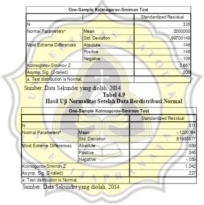
Tabel 4.8
Hasil Uji Normalitas dengan Kolmogorov Smirnov Sebelum Data Normal
Sumber: Data Sekunder yang diolah, 2014
Tabel 4.9
Hasil Uji Normalitas Setelah Data Berdistribusi Normal
Sumber: Data Sekunder yang diolah, 2014.
One-Sample Kolmogorov-Smirnov Test
Standardized Residual
N 335
Normal Parametersa Mean .0000000
Std. Deviation .99700149
Most Extreme Differences Absolute .146
Positive .146
Negative -.106
Kolmogorov-Smirnov Z 2.667
Asymp. Sig. (2-tailed) .000
a. Test distribution is Normal.
One-Sample Kolmogorov-Smirnov Test
Standardized Residual
N 311
Normal Parametersa Mean -.1200764
Std. Deviation .61903877
Most Extreme Differences Absolute .059
Positive .045
Negative -.059
Kolmogorov-Smirnov Z 1.042
Asymp. Sig. (2-tailed) .227
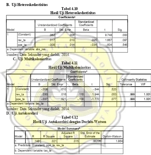
B. Uji Heteroskedastisitas
Tabel 4.10
Hasil Uji Heteroskedastisitas
CoefficientsaModel
Unstandardized Coefficients
Standardized Coefficients
t Sig.
B Std. Error Beta
1 (Constant) .062 .006
9.748 .000
rev_ta .017 .010 .095 1.667 .097
ppe_ta -.008 .014 -.034 -.604 .546
a. Dependent Variable: abs_res
Sumber: Data Sekunder yang diolah, 2014.
C. Uji Multikolonieritas
Tabel 4.11
Hasil Uji Multikoloniaritas
CoefficientsaModel
Unstandardized Coefficients
Standardized Coefficients
t Sig.
Collinearity Statistics
B Std. Error Beta Tolerance VIF
1 (Constant) -.006 .010 -.644 .520
rev_ta .030 .016 .110 1.944 .053 .999 1.001
ppe_ta -.037 .021 -.100 -1.772 .077 .999 1.001
a. Dependent Variable: tac_ta
Sumber: Data Sekunder yang diolah, 2014.
D. Uji Autokorelasi
Tabel 4.12
Hasil Uji Autokorelasi dengan Durbin-Watson
Sumber: Data Sekunder yang diolah, 2014.
Model Summaryb
Model R R Square
Adjusted R Square
Std. Error of the
Estimate Durbin-Watson
1 .146a .021 .015 .08206 1.864
a. Predictors: (Constant), ppe_ta, rev_ta
REGRESI AKRUAL DISKRESIONER
Regression
Notes
Output Created 03-May-2014 07:54:20
Comments
Input Data E:\skripsi berna\311 data ke 281.sav
Active Dataset DataSet1
Filter <none>
Weight <none>
Split File <none>
N of Rows in Working Data File 281
Missing Value Handling Definition of Missing User-defined missing values are treated as
missing.
Cases Used Statistics are based on cases with no
missing values for any variable used.
Syntax REGRESSION
/MISSING LISTWISE
/STATISTICS COEFF OUTS R ANOVA COLLIN TOL
/CRITERIA=PIN(.05) POUT(.10) /NOORIGIN
/DEPENDENT DA
/METHOD=ENTER KAP SIZE LEV CFO SALES_Grw LAG_LOSS
/RESIDUALS DURBIN.
Resources Processor Time 00:00:00.265
Elapsed Time 00:00:00.156
Memory Required 3188 bytes
Additional Memory Required for
Residual Plots 0 bytes
[DataSet1] E:\skripsi berna\311 data ke 281.sav
Variables Entered/Removedb
Model Variables Entered
Variables
Removed Method
1 LAG_LOSS, KAP,
SALES_Grw, LEV,
CFO, SIZEa
. Enter
a. All requested variables entered.
Model Summaryb
Model R R Square Adjusted R Square
Std. Error of the
Estimate Durbin-Watson
1 .216a .047 .026 .0358527 1.904
a. Predictors: (Constant), LAG_LOSS, KAP, SALES_Grw, LEV, CFO, SIZE
b. Dependent Variable: DA
ANOVAb
Model Sum of Squares df Mean Square F Sig.
1 Regression .017 6 .003 2.231 .040a
Residual .352 274 .001
Total .369 280
a. Predictors: (Constant), LAG_LOSS, KAP, SALES_Grw, LEV, CFO, SIZE
b. Dependent Variable: DA
Coefficientsa
Model
Unstandardized Coefficients
Standardized Coefficients
t Sig.
Collinearity Statistics
B Std. Error Beta Tolerance VIF
1 (Constant) .110 .041
2.647 .009
KAP .010 .005 .135 1.858 .064 .661 1.513
SIZE -.006 .003 -.120 -1.679 .094 .686 1.457
LEV .009 .005 .125 2.035 .043 .919 1.088
CFO -.016 .021 -.051 -.768 .443 .774 1.292
SALES_Grw .002 .009 .016 .266 .790 .944 1.059
LAG_LOSS .008 .007 .072 1.159 .247 .909 1.100
Collinearity Diagnosticsa
Model Dimen
sion Eigenvalue
Condition Index
Variance Proportions
(Constant) KAP SIZE LEV CFO
SALES_
Grw LAG_LOSS
1 1 3.931 1.000 .00 .01 .00 .02 .02 .01 .01
2 1.104 1.887 .00 .03 .00 .04 .04 .13 .38
3 .747 2.294 .00 .07 .00 .00 .08 .74 .04
4 .640 2.478 .00 .10 .00 .20 .04 .03 .49
5 .338 3.408 .00 .60 .00 .03 .63 .00 .02
6 .238 4.062 .00 .02 .00 .69 .20 .07 .02
7 .001 54.492 1.00 .16 1.00 .02 .00 .01 .05
a. Dependent Variable: DA
Residuals Statisticsa
Minimum Maximum Mean Std. Deviation N
Predicted Value .036026 .078154 .047908 .0078395 281
Residual
-6.5734245E-2 .0959301 .0000000 .0354665 281
Std. Predicted Value -1.516 3.858 .000 1.000 281
Std. Residual -1.833 2.676 .000 .989 281
a. Dependent Variable: DA
1.2 Menghitung
Discresionary accruals
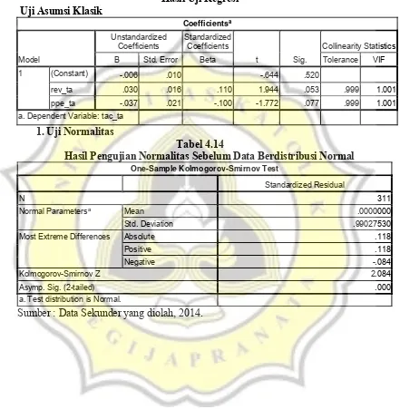
Tabel 4.13
Hasil Uji Regresi
Uji Asumsi Klasik
1. Uji Normalitas
Tabel 4.14
Hasil Pengujian Normalitas Sebelum Data Berdistribusi Normal
One-Sample Kolmogorov-Smirnov Test
Standardized Residual
N 311
Normal Parametersa Mean .0000000
Std. Deviation .99027530
Most Extreme Differences Absolute .118
Positive .118
Negative -.084
Kolmogorov-Smirnov Z 2.084
Asymp. Sig. (2-tailed) .000
a. Test distribution is Normal.
Sumber : Data Sekunder yang diolah, 2014.
Coefficientsa
Model
Unstandardized Coefficients
Standardized Coefficients
t Sig.
Collinearity Statistics
B Std. Error Beta Tolerance VIF
1 (Constant) -.006 .010
-.644 .520
rev_ta .030 .016 .110 1.944 .053 .999 1.001
ppe_ta -.037 .021 -.100 -1.772 .077 .999 1.001
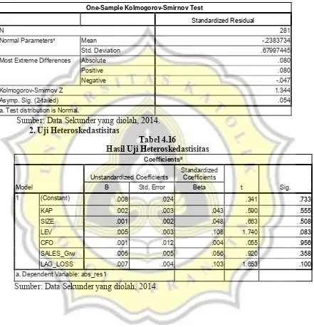
Tabel 4. 15
Hasil Uji Normalitas Setelah Data Berdistribusi Normal
Sumber: Data Sekunder yang diolah, 2014.
2. Uji Heteroskedastisitas
Tabel 4.16
Hasil Uji Heteroskedastisitas
CoefficientsaModel
Unstandardized Coefficients
Standardized Coefficients
t Sig.
B Std. Error Beta
1 (Constant) .008 .024
.341 .733
KAP .002 .003 .043 .590 .555
SIZE .001 .002 .048 .663 .508
LEV .005 .003 .108 1.740 .083
CFO .001 .012 .004 .055 .956
SALES_Grw .005 .005 .056 .920 .358
LAG_LOSS .007 .004 .103 1.653 .100
a. Dependent Variable: abs_res1
Sumber: Data Sekunder yang diolah, 2014.
One-Sample Kolmogorov-Smirnov Test
Standardized Residual
N 281
Normal Parametersa Mean -.2383734
Std. Deviation .67997445
Most Extreme Differences Absolute .080
Positive .080
Negative -.047
Kolmogorov-Smirnov Z 1.344
Asymp. Sig. (2-tailed) .054
3. Uji Autokorelasi Uji Multikolonieritas
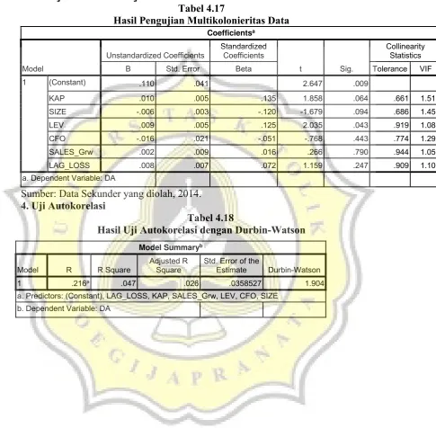
Tabel 4.17
Hasil Pengujian Multikolonieritas Data
CoefficientsaModel
Unstandardized Coefficients
Standardized Coefficients
t Sig.
Collinearity Statistics
B Std. Error Beta Tolerance VIF
1 (Constant) .110 .041
2.647 .009
KAP .010 .005 .135 1.858 .064 .661 1.513
SIZE -.006 .003 -.120 -1.679 .094 .686 1.457
LEV .009 .005 .125 2.035 .043 .919 1.088
CFO -.016 .021 -.051 -.768 .443 .774 1.292
SALES_Grw .002 .009 .016 .266 .790 .944 1.059
LAG_LOSS .008 .007 .072 1.159 .247 .909 1.100
a. Dependent Variable: DA
Sumber: Data Sekunder yang diolah, 2014.
4. Uji Autokorelasi
Tabel 4.18
Hasil Uji Autokorelasi dengan Durbin-Watson
Model Summaryb
Model R R Square
Adjusted R Square
Std. Error of the
Estimate Durbin-Watson
1 .216a .047 .026 .0358527 1.904
a. Predictors: (Constant), LAG_LOSS, KAP, SALES_Grw, LEV, CFO, SIZE
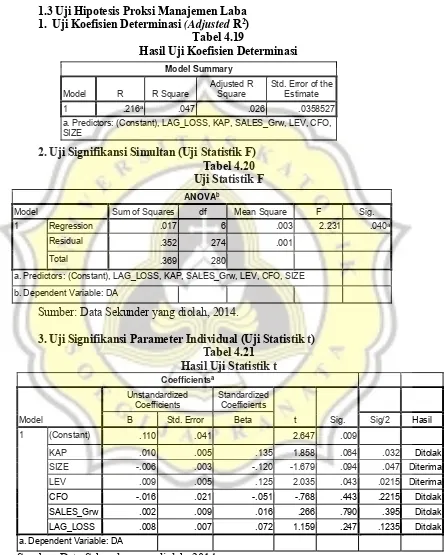
1.3 Uji Hipotesis Proksi Manajemen Laba
1. Uji Koefisien Determinasi
(Adjusted
R
2)
Tabel 4.19
Hasil Uji Koefisien Determinasi
2. Uji Signifikansi Simultan (Uji Statistik F)
Tabel 4.20
Uji Statistik F
Sumber: Data Sekunder yang diolah, 2014.
3. Uji Signifikansi Parameter Individual (Uji Statistik t)
Tabel 4.21
Hasil Uji Statistik t
CoefficientsaModel
Unstandardized Coefficients
Standardized Coefficients
t Sig.
B Std. Error Beta Sig/2 Hasil
1 (Constant) .110 .041
2.647 .009
KAP .010 .005 .135 1.858 .064 .032 Ditolak
SIZE -.006 .003 -.120 -1.679 .094 .047 Diterima
LEV .009 .005 .125 2.035 .043 .0215 Diterima
CFO -.016 .021 -.051 -.768 .443 .2215 Ditolak
SALES_Grw .002 .009 .016 .266 .790 .395 Ditolak
LAG_LOSS .008 .007 .072 1.159 .247 .1235 Ditolak
a. Dependent Variable: DA
Sumber: Data Sekunder yang diolah, 2014.
Model Summary
Model R R Square
Adjusted R Square
Std. Error of the Estimate
1 .216a .047 .026 .0358527
a. Predictors: (Constant), LAG_LOSS, KAP, SALES_Grw, LEV, CFO, SIZE
ANOVAb
Model Sum of Squares df Mean Square F Sig.
1 Regression .017 6 .003 2.231 .040a
Residual .352 274 .001
Total .369 280
a. Predictors: (Constant), LAG_LOSS, KAP, SALES_Grw, LEV, CFO, SIZE
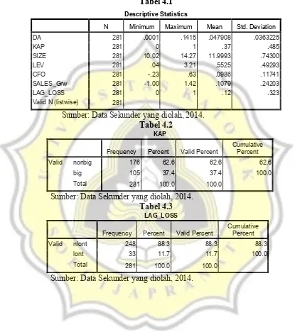
1.4 Analisis Statistik Deskriptif Proksi Manajemen Laba
Tabel 4.1
Sumber: Data Sekunder yang diolah, 2014.
Tabel 4.2
KAPFrequency Percent Valid Percent
Cumulative Percent
Valid nonbig 176 62.6 62.6 62.6
big 105 37.4 37.4 100.0
Total 281 100.0 100.0
Sumber: Data Sekunder yang diolah, 2014.
Tabel 4.3
LAG_LOSSFrequency Percent Valid Percent
Cumulative Percent
Valid nlont 248 88.3 88.3 88.3
lont 33 11.7 11.7 100.0
Total 281 100.0 100.0
Sumber: Data Sekunder yang diolah, 2014.
Descriptive Statistics
N Minimum Maximum Mean Std. Deviation
DA 281 .0001 .1415 .047908 .0363225
KAP 281 0 1 .37 .485
SIZE 281 10.02 14.27 11.9993 .74300
LEV 281 .04 3.21 .5525 .49293
CFO 281 -.23 .63 .0986 .11741
SALES_Grw 281 -1.00 1.42 .1079 .24203
LAG_LOSS 281 0 1 .12 .323
Logistic Regression
Notes
Output Created 03-May-2014 08:29:03
Comments
Input Data E:\skripsi data\311 data ke 281.sav
Active Dataset DataSet1
Filter <none>
Weight <none>
Split File <none>
N of Rows in Working Data File 281
Missing Value Handling Definition of Missing User-defined missing values are treated as
missing
Syntax LOGISTIC REGRESSION VARIABLES GO
/METHOD=ENTER KAP SIZE LEV CFO SALES_Grw LAG_LOSS
/CLASSPLOT
/PRINT=GOODFIT CORR ITER(1) /CRITERIA=PIN(0.05) POUT(0.10) ITERATE(20) CUT(0.5).
Resources Processor Time 00:00:00.078
Elapsed Time 00:00:00.187
[DataSet1] E:\skripsi data\311 data ke 281.sav
Case Processing Summary
Unweighted Casesa N Percent
Selected Cases Included in Analysis 281 100.0
Missing Cases 0 .0
Total 281 100.0
Unselected Cases 0 .0
Total 281 100.0
a. If weight is in effect, see classification table for the total number of cases.
Dependent Variable Encoding Original
Value Internal Value
Ngcao 0
Block 0: Beginning Block
Iteration Historya,b,c
Iteration -2 Log likelihood
Coefficients
Constant
Step 0 1 207.563 -1.544
2 199.439 -1.972
3 199.257 -2.049
4 199.257 -2.052
5 199.257 -2.052
a. Constant is included in the model.
b. Initial -2 Log Likelihood: 199.257
c. Estimation terminated at iteration number 5 because parameter estimates changed by less than .001.
Classification Tablea,b
Observed
Predicted
GO
Percentage Correct
ngcao gcao
Step 0 GO ngcao 249 0 100.0
gcao 32 0 .0
Overall Percentage
88.6
a. Constant is included in the model.
b. The cut value is .500
Variables in the Equation
B S.E. Wald df Sig. Exp(B)
Step 0 Constant -2.052 .188 119.365 1 .000 .129
Variables not in the Equation
Score df Sig.
Step 0 Variables KAP 3.703 1 .054
SIZE 22.375 1 .000
Block 1: Method = Enter
Iteration Historya,b,c,d
Iteration
-2 Log likelihood
Coefficients
Constant KAP SIZE LEV CFO SALES_Grw LAG_LOSS
Step 1 1 141.535 -.411 .217 -.160 1.254 -.943 -.428 1.267
2 110.228 -.175 .364 -.269 1.891 -2.313 -.794 1.942
3 103.849 .157 .429 -.344 2.248 -4.076 -1.084 2.314
4 103.131 .351 .414 -.375 2.361 -5.305 -1.191 2.438
5 103.113 .392 .403 -.380 2.377 -5.576 -1.203 2.455
6 103.113 .394 .403 -.380 2.377 -5.585 -1.203 2.455
7 103.113 .394 .403 -.380 2.377 -5.585 -1.203 2.455
a. Method: Enter
b. Constant is included in the model.
c. Initial -2 Log Likelihood: 199.257
d. Estimation terminated at iteration number 7 because parameter estimates changed by less
than .001.
Omnibus Tests of Model Coefficients
Chi-square df Sig.
Step 1 Step 96.144 6 .000
Block 96.144 6 .000
Model 96.144 6 .000
Model Summary
Step -2 Log likelihood
Cox & Snell R Square
Nagelkerke R Square
1 103.113a .290 .570
a. Estimation terminated at iteration number 7 because parameter estimates changed by less than .001.
Hosmer and Lemeshow Test
Step Chi-square df Sig.
Contingency Table for Hosmer and Lemeshow Test
GO = ngcao GO = gcao
Total
Observed Expected Observed Expected
Step 1 1 28 27.846 0 .154 28
2 28 27.708 0 .292 28
3 28 27.594 0 .406 28
4 28 27.444 0 .556 28
5 28 27.288 0 .712 28
6 28 27.109 0 .891 28
7 24 26.868 4 1.132 28
8 26 26.359 2 1.641 28
9 22 23.021 6 4.979 28
10 9 7.763 20 21.237 29
Classification Tablea
Observed
Predicted
GO
Percentage Correct
ngcao gcao
Step 1 GO ngcao 243 6 97.6
gcao 13 19 59.4
Overall Percentage
93.2
a. The cut value is .500
Variables in the Equation
B S.E. Wald df Sig. Exp(B)
Step 1a KAP .403 .611 .434 1 .510 1.496
SIZE -.380 .435 .764 1 .382 .684
LEV 2.377 .564 17.769 1 .000 10.776
CFO -5.585 3.173 3.098 1 .078 .004
SALES_Grw -1.203 .987 1.487 1 .223 .300
LAG_LOSS 2.455 .580 17.939 1 .000 11.646
Constant .394 5.197 .006 1 .940 1.482
Correlation Matrix
Constant KAP SIZE LEV CFO SALES_Grw LAG_LOSS
Step 1 Constant 1.000 .179 -.994 -.268 .072 .153 -.336
KAP .179 1.000 -.211 -.011 -.157 -.044 -.082
SIZE -.994 -.211 1.000 .189 -.100 -.160 .282
LEV -.268 -.011 .189 1.000 .083 .009 .208
CFO .072 -.157 -.100 .083 1.000 -.032 .096
SALES_Grw .153 -.044 -.160 .009 -.032 1.000 .033
LAG_LOSS -.336 -.082 .282 .208 .096 .033 1.000
Step number: 1
Observed Groups and Predicted Probabilities
80 ┼ ┼ │ │ │ │ F │ │ R 60 ┼ n ┼ E │ nn │ Q │ nn │ U │ nn │ E 40 ┼ nn ┼ N │nnng │ C │nnnn │ Y │nnnn │ 20 ┼nnnng ┼ │nnnnn │ │nnnnnn │ │nnnnnnnnng n g g g │
Predicted ───────── ───────── ───────── ───────── ───────── ───────── ───────── ───────── ───┼ ┼ ┼ ┼ ┼ ┼ ┼ ┼
┼
────── ──────────
Prob: 0 .1 .2 .3 .4 .5 .6 .7 .8 .9 1
Group: nnnnnnnnnnnnnnnnnnnnnnnnnnnnnnnnnnnnnnnnnnnnnnnnnnggggggggggggggggggggggggggggggggg ggggggggggggggggg
Predicted Probability is of Membership for gcao The Cut Value is .50
Symbols: n ‐ ngcao g ‐ gcao
Each Symbol Represents 5 Cases.
Menghitung Kualitas Audit Proksi Opini Audit
Going Concern
1. Analisis Data Logit
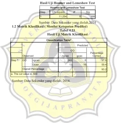
1.1 Menilai Kelayakan Model Regresi
Tabel 4.22
Hasil Uji Hosmer and Lemeshow Test
Sumber: Data Sekunder yang diolah,2014
1.2 Matrik Klasifikasi ( Menilai Ketepatan Prediksi
)
Tabel 4.23
Hasil Uji Matrik Klasifikasi
Sumber: Data Sekunder yang diolah, 2014.
Hosmer and Lemeshow Test
Step Chi-square df Sig.
1 11.254 8 .188
Classification Tablea
Observed
Predicted
GO
Percentage Correct
ngcao gcao
Step 1 GO ngcao 243 6 97.6
Gcao 13 19 59.4
Overall Percentage
93.2
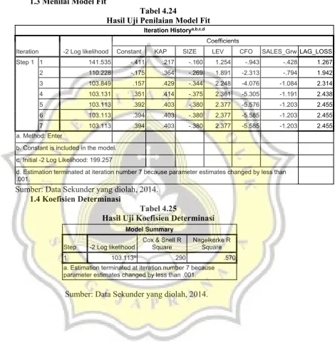
1.3 Menilai Model Fit
Tabel 4.24
Hasil Uji Penilaian Model Fit
Iteration Historya,b,c,dIteration -2 Log likelihood
Coefficients
Constant KAP SIZE LEV CFO SALES_Grw LAG_LOSS
Step 1 1 141.535 -.411 .217 -.160 1.254 -.943 -.428 1.267
2 110.228 -.175 .364 -.269 1.891 -2.313 -.794 1.942
3 103.849 .157 .429 -.344 2.248 -4.076 -1.084 2.314
4 103.131 .351 .414 -.375 2.361 -5.305 -1.191 2.438
5 103.113 .392 .403 -.380 2.377 -5.576 -1.203 2.455
6 103.113 .394 .403 -.380 2.377 -5.585 -1.203 2.455
7 103.113 .394 .403 -.380 2.377 -5.585 -1.203 2.455
a. Method: Enter
b. Constant is included in the model.
c. Initial -2 Log Likelihood: 199.257
d. Estimation terminated at iteration number 7 because parameter estimates changed by less than
.001.
Sumber: Data Sekunder yang diolah, 2014.
1.4 Koefisien Determinasi
Tabel 4.25
Hasil Uji Koefisien Determinasi
Sumber: Data Sekunder yang diolah, 2014.
Model Summary
Step -2 Log likelihood
Cox & Snell R Square
Nagelkerke R Square
1 103.113a .290 .570
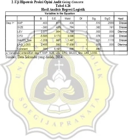
2 .Uji Hipotesis Proksi Opini Audit
Going Concern
Tabel 4.26
Hasil Analisis Regresi Logistik
Variables in the Equation
B S.E. Wald Df Sig. Sig/2 Hasil
Step 1a KAP .403 .611 .434 1 .510 .2555 Ditolak
SIZE -.380 .435 .764 1 .382 .191 Ditolak
LEV 2.377 .564 17.769 1 .000 .000 Diterima
CFO -5.585 3.173 3.098 1 .078 .039 Ditolak
SALES_Grw -1.203 .987 1.487 1 .223 .1115 Ditolak
LAG_LOSS 2.455 .580 17.939 1 .000 .000 Diterima
Constant .394 5.197 .006 1 .940
a. Variable(s) entered on step 1: KAP, SIZE, LEV, CFO, SALES_Grw, LAG_LOSS.
3. Analisis Statistik Deskriptif Proksi Opini Audit
Going Concern
Tabel 4.4
Sumber: Data Sekunder yang diolah, 2014.
Tabel 4.5
GOING CONCERNFrequency Percent Valid Percent
Cumulative Percent
Valid ngcao 249 88.6 88.6 88.6
gcao 32 11.4 11.4 100.0
Total 281 100.0 100.0
Sumber: Data Sekunder yang diolah, 2014.
Tabel 4.6
KAPFrequency Percent Valid Percent
Cumulative Percent
Valid nonbig 176 62.6 62.6 62.6
big 105 37.4 37.4 100.0
Total 281 100.0 100.0
Sumber: Data Sekunder yang diolah, 2014.
Tabel 4.7
LAG_LOSSFrequency Percent Valid Percent
Cumulative Percent
Valid nlont 248 88.3 88.3 88.3
lont 33 11.7 11.7 100.0
Total 281 100.0 100.0
Descriptive Statistics
N Minimum Maximum Mean Std. Deviation
GO 281 0 1 .11 .318
KAP 281 0 1 .37 .485
SIZE 281 10.02 14.27 11.9993 .74300
LEV 281 .04 3.21 .5525 .49293
CFO 281 -.23 .63 .0986 .11741
SALES_Grw 281 -1.00 1.42 .1079 .24203
LAG_LOSS 281 0 1 .12 .323