T H E J O U R N A L O F H U M A N R E S O U R C E S • 47 • 3
Weaker
Prenatal Pollution Exposure and Educational
Outcomes
Nicholas J. Sanders
A B S T R A C T
I examine the impact of prenatal total suspended particulate (TSP) expo-sure on educational outcomes using county-level variation in the timing and severity of the industrial recession of the early 1980s as a shock to ambient TSPs (similar to Chay and Greenstone 2003b). I then instrument for pollution levels using county-level changes in relative manufacturing employment. A standard deviation decrease in TSPs in a student’s year of birth is associated with 2 percent of a standard deviation increase in high school test scores for OLS and 6 percent for IV. I also consider how mi-gration and selection into motherhood relate to my results.
I. Introduction
The fetal origins hypothesis (FOH) suggests that the “kind and qual-ity of nutrition [we] received in the womb; the pollutants, drugs and infections [we] were exposed to during gestation . . . shape our susceptibility to disease, our appetite and metabolism, our intelligence and temperament.” (Paul 2010b) Almond and Cur-rie (2011) recently reviewed the steps economists have taken to cleanly identify the validity of the FOH, and provided substantial evidence that impacts of in utero treatments can continue to play out later in life. The FOH raises an interesting suggestion thatin uteropollution exposure could carry long-term consequences such
Nicholas J. Sanders is an assistant professor of economics at the College of William & Mary, but com-pleted this research as a postdoctoral fellow at the Stanford Institute for Economic Policy Research, Stanford University. He thanks Hilary Hoynes, Christopher R. Knittel, Douglas L. Miller, Jed T. Richard-son, and seminar participants at the All University of California Labor Conference, the University of California, Davis, Sacramento State University, Sonoma State University, Lewis & Clark College, Uni-versity of Tennessee, Williams College, Stanford UniUni-versity, the Atmospheric Aerosols & Health Group, the NBER Summer Institute, the NBER Labor Meetings, and the SIEPR Postdoc Conference for helpful comments. Student-level data used in this analysis contain year of birth, information that is not publicly provided by the Texas Education Agency. It is, however, available for purchase upon request. The author may be contacted for further details at < njsanders@wm.edu > .
as decreased performance in school, lower educational attainment, and reduced earn-ings and lifespan. And while some impacts ofin utero pollution on developmental factors may be observed using current metrics of infant health, factors with direct mental impacts that are unaccompanied by commonly observed physical traits go uncounted, and policy decisions made solely on the basis of contemporaneously observed physical measures may be understating the true costs of pollution.
Economists have found a number of pollutants to be hazardous to contempora-neous physical health.1Less is known about how impacts extend further in the life cycle, though recent research finds higher lead levels lower IQ scores and increase deviant behavior as well as decrease educational performance, cognitive ability, and labor market outcomes (Reyes 2007; Nilsson 2009), and prenatal radiation exposure lowers later test scores (Almond, Edlund, and Palme 2009). I further the research on pollution and health by considering the impacts of prenatal total suspended par-ticulate matter (TSP) exposure on long-run outcomes, specifically educational achievement in high school. Unlike prior research on pollution and long-run events, I examine a common, currently regulated pollutant that remains ubiquitous even under today’s more strict environmental policies. And while a good deal has been learned about the negative health effects of particulates, little is known about how such a pollutant might impact mental development and cognitive ability. Given the ever-present debate over regulatory policy, such considerations are of drastic im-portance.
I combine several data sets containing economic, demographic, weather, pollution, and test information from the state of Texas and exploit a period of industrial re-cession in Texas from 1981 to 1983 with its dramatic impact on manufacturing production and associated ambient TSP levels, similar to the identification strategy first employed in Chay and Greenstone (2003b). Ordinary least squares (OLS) show that, during the recessionary period, a standard-deviation decrease in the mean pol-lution level in a child’s year of birth is associated with 2 percent of a standard deviation increase in high school test performance. As a correction for potential complications such as measurement error and omitted variables bias, I then instru-ment for TSPs using annual employinstru-ment changes in the county-level manufacturing sector. Instrumental variables (IV) results are larger; a standard deviation decrease in TSPs is associated with approximately 6 percent of a within-county standard deviation increase in test performance. Results are statistically significant only in the years of greatest pollution variation, suggesting that the effect may be too subtle to identify using mild changes in ambient pollution caused by time variation or by making across-county cross-sectional comparisons. I also discuss challenges to iden-tification including measurement error, systematic migration, and selection into motherhood and health behavior, and how each may bias my results.
Section II provides scientific background on the relationship between particulate matter and brain development. Section III describes the data. Section IV discusses
the intuition behind the period of analysis, choice of instrument and some potential complications to identification. Section V describes the empirical methods used. Section VI presents my results. Section VII considers additional factors important in the interpretation of my results. Section VIII concludes.
II. Pollution, health, and intrauterine development
I focus on airborne TSPs, the measure of particulate pollution used by the EPA in the earlier years of the Clean Air Act and up through the late 1980s. This includes all suspended, airborne liquid or solid particles smaller than 100 mi-crometers in size. Suspended particulates can be naturally occurring (for example, dust, dirt, and pollen), which tend to make up the larger particles, and a byproduct of common economic activities such as fuel combustion (for example, coal, gasoline and diesel), fires, and industrial activity, which tend to make up the smaller particles. Regulatory attention has shifted to finer sizes of particulate matter, smaller than 10 micrometers (PM10) and smaller than 2.5 micrometers (PM2.5). Both of these size classifications are contained with the older TSP measure. As the composition of particular matter varies, there is no scientifically identified conversion metric be-tween TSP levels and the more modern measures. However, it is useful to consider such a relationship given that much of the work in economics today uses the PM10 classification. A 1999 study by the World Bank Group noted a commonly used ratio is PM10 = TSP∗0.55 (The World Bank Group 1999).
Inhaled particulates cause a number of health problems including difficulty breath-ing, decreased lung function, aggravated asthma, and cardiac trouble. Exactly how particulates might impact health depends partially on their size, which influences how the body responds to exposure. Particles can be classified as inhalable, thoracic, and respirable based on their expected deposition. Larger particles (inhalable) are more likely to cause physical problems in the mouth, nose, and trachea, both in the short term (for example, difficulty breathing) and the long term (for example, nasal and esophageal cancer). Particles that are small enough to enter the lungs can do damage to the lung tissue. Particles smaller than 4µm are respirable, and can pen-etrate to the level of alveoli and interfere with oxygen gas exchange (EPA 2009).
birth weight. For (1), low birth weight is currently observed and can be considered in formation of policy. For (2), my results suggest consideration of low birth weight alone will underestimate the true social costs of pollution.
Research on finer particles suggests particulate matter may indeed alter fetal de-velopment in manners less easily observed. For example, Perera, Li, Whyatt, Hoep-ner, Wang, Camann, and Rauh (2009) found a link between fuel-combustion related polycyclic aromatic hydrocarbons (PAHs), a specific type of particulate matter, and a number of pre- and early postnatal developmental problems including damage to the immune system, hindered neurological development, impairment of neuron be-havior associated with long-term memory formation, and lower IQ scores at age 5. They found no statistically significant difference in birth weight or gestation length, suggesting such mental effects can be present even when observable physical effects are not. Other medical studies have found correlations between air pollution and brain damage, including cerebral vascular damage, neuroinflammation, neurodegen-eration (Block and Caldero´n-Garciduen˜as 2009), and brain legions (Raloff 2010). Controlled studies on rats found those exposed to fine and ultrafine particles had elevated proinflammatory response in their brain tissue (Campbell, Oldham, Becaria, Bondy, Meacher, Sioutas, Misra, Mendez, and Kleinman 2005), and that long-run PM2.5 exposure led to decreased cognition and observable brain differences such as fewer dendrites and reduced cell complexity (Fonken, Xu, Weil, Chen, Sun, Ra-jagopalan and Nelson 2011). Observational studies of children exposed to black carbon found higher levels of pollution exposure were associated with lower memory and cognition even after controlling for birth weight, sociodemographics, tobacco smoke exposure, and blood lead level (Suglia, Gryparis, Wright, Schwartz, and Wright 2008).
While these studies are not focused on in utero exposure, they suggest a link between particulates and brain damage. More specificin utero-driven mental effects have been detected for exposure to methymercury, another form of particulate (Grandjean, Weihe, White, and Debes 1998; Debes, Budtz-Jørgensen, Weihe, White, and Grandjean 2006), and controlled studies using rats foundin uteroexposure to diesel exhaust, a major source of particulate matter, resulted in decreased locomotor activity and altered neurochemistry in the brain (Suzuki, Oshio, Iwata, Saburi, Oda-giri, Udagawa, Sugawara, Umezawa, and Takeda 2010).
In summary, particulate matter could have lasting impacts on mental ability via a number of fetal mechanisms. Larger particles are likely to cause health problems in the mother, which could then harm fetal development. Based on prior research, such impacts are likely to be accompanied by physically observable damages such as premature birth and lower birth weight. But smaller particles, which have the ability to permeate protective membranes, could cause damage to fetal neural cells without physical damages that would be observed in commonly measured indicators of infant health.
III. Data
arith-metic mean come from the EPA database of historical air quality data. Readings from all pollution monitors within 20 miles of a county population centroid are collapsed to an annual mean and weighted by the inverse of their distance from said centroid. Thirty counties have population centroids within 20 miles of at least one monitor active for all years from 1979–85.2I use only monitors that take readings regularly over the year (at least one an average of every two weeks) so as not to have any one period on the year influence my results.3 Results were similar using all available monitors without restrictions, though the first stage was slightly weaker due to decreased precision of pollution measurement.
Weather is a potential confounder in the regression of student test outcomes on pollution exposure due to health interactions (Descheˆnes and Greenstone 2007; Bar-reca 2008; Descheˆnes, Greenstone and Guryan 2009; Stoecker 2010) and my first-stage regression (see Knittel, Miller and Sanders (2009) for an in-depth discussion of weather and pollution). Using data from the Global Surface Summary of the day, I control for third-order polynomials in average annual temperature, number of days with rain, and average annual specific humidity. To get county level measures I follow a strategy similar to my pollution data, but allow for inclusion of all monitors within 50 miles due to the substantially smaller number of weather monitors present. In some specifications I allow for more nonparametric weather controls and consider wind speed as well. Yearly averages by birth year cohorts for pollution and weather variables are shown in Table 1.
Industry level employment estimates (used for instrument construction as de-scribed in Section V), and per capita income are from the Regional Economic In-formation System (REIS). I also use the REIS annual population estimates and Cen-sus land area information to construct a county by year population density estimate to control for urbanization and its impact on both pollution levels and education.
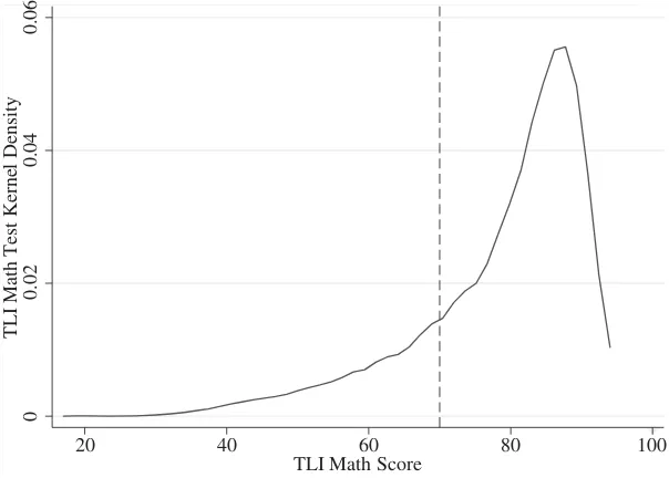
Test score data are from the Texas Education Agency (TEA) monitored Texas Assessment of Academic Skills (TAAS). From 1994 to 2002, tenth graders were required to exhibit competency on both a TAAS math exam and reading exam, where competency is a score of 70 or higher on the Texas Learning Index (TLI), an annually adjusted score intended to equate difficulty of passing across test years.4 Students who have not achieved competency by twelfth grade cannot graduate from high school, making the TAAS a high stakes exam. Note that, while I only use the score from each student’s first tenth grade attempt, they have additional opportunities in eleventh and twelfth grade to retake the exam if necessary. I focus on the math portion of the exam as an outcome variable, as math scores are often considered more informative of learning when discussing standardized exams and used more frequently in the education literature.5Figure 1 shows the distribution of the first-attempt test scores with an indicator line for the passing score of 70.
2. I have repeated my analysis using distances of 10 and 30 miles, and results are largely similar across distance choice. These results are not included but are available upon request.
3. Monitors that take few readings per year have a disproportionately large number of readings taken during the winter.
4. See Martorell (2004) for a more detailed discussion of the TAAS exit exams, and Haney (2000) for discussion of difficulty of the exam across test years.
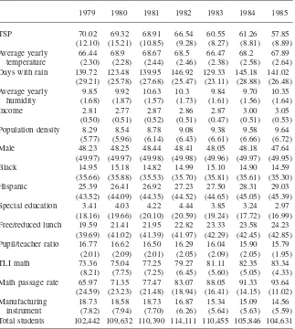
Table 1
Annual Means and Standard Deviations
1979 1980 1981 1982 1983 1984 1985
TSP 70.02 69.32 68.91 66.54 60.55 61.26 57.85
(12.10) (15.21) (10.85) (9.28) (8.27) (8.81) (8.89) Average yearly
temperature
66.44 68.9 68.67 68.5 66.47 68.2 67.89 (2.30) (2.28) (2.44) (2.46) (2.38) (2.58) (2.64) Days with rain 139.72 123.48 139.95 146.92 129.33 145.18 141.02
(29.21) (25.78) (27.68) (25.47) (23.11) (28.88) (26.48) Average yearly
humidity
9.85 9.92 10.63 10.3 9.84 9.70 10.35 (1.68) (1.87) (1.57) (1.73) (1.61) (1.56) (1.64)
Income 2.81 2.77 2.87 2.86 2.87 3.00 3.05
(0.50) (0.51) (0.52) (0.51) (0.47) (0.51) (0.53) Population density 8.29 8.54 8.78 9.08 9.38 9.58 9.64
(5.77) (5.96) (6.14) (6.43) (6.61) (6.66) (6.72)
Male 48.23 48.25 48.44 48.41 48.05 48.18 47.64
(49.97) (49.97) (49.98) (49.98) (49.96) (49.97) (49.95)
Black 14.95 15.18 14.82 14.99 15.10 14.90 14.59
(35.66) (35.88) (35.53) (35.70) (35.81) (35.61) (35.30) Hispanic 25.39 26.41 26.92 27.23 27.50 28.31 29.03
(43.52) (44.09) (44.35) (44.52) (44.65) (45.05) (45.39) Special education 3.41 4.03 4.22 4.44 3.85 3.24 2.97
(18.16) (19.66) (20.10) (20.59) (19.24) (17.72) (16.99) Free/reduced lunch 19.59 21.41 21.95 22.82 23.33 23.58 24.23
(39.69) (41.02) (41.39) (41.97) (42.29) (42.45) (42.85) Pupil/teacher ratio 16.77 16.62 16.50 16.29 16.04 15.90 15.79
(2.01) (2.09) (2.01) (2.05) (2.09) (2.05) (1.95) TLI math 73.36 75.04 77.25 79.27 81.11 82.35 83.34
(8.21) (7.75) (7.25) (6.45) (5.60) (5.05) (4.33) Math passage rate 65.97 71.35 77.47 83.07 88.05 91.33 93.64
(24.59) (23.23) (21.48) (18.94) (16.41) (14.15) (11.02) Manufacturing
instrument
18.73 18.58 18.73 16.87 15.34 15.09 14.56 (7.82) (7.94) (7.70) (6.26) (5.64) (5.63) (5.59) Total students 102,442 109,632 110,390 114,111 110,455 105,846 104,631
Notes: Standard deviations shown in parenthesis. Years shown are year of birth, with test-taking years ranging from 1994 to 2002. Data are for all students with nonmissing covariates and calculated age at test taking between 15 and 18 years of age. Population density is persons per square mile over 100. Data are described in detail in Section III.
20 40 60 80 100 TLI Math Score
0
0.02
0.04
0.06
TLI Math Test Kernel Density
Figure 1
Kernel Density for Texas Learning Index Math Scores
Notes: Kernel density calculated using a bandwidth of two. Dashed line indicates the passing cutoff of 70. Distribution calculated using all students in the main analysis. TLI stands for “Texas Learning Index,” a difficulty-weighted scoring metric designed to maintain consistency in test scoring across testing cohorts.
for the population makeup of the counties and partially control for differences in outcomes spanning from variation in overall racial and ethnic makeup across regions. The majority of students taking exit exams between 1994 and 2002 have years of birth between 1979 and 1985, allowing me to view birth cohorts in a period before the recession (1979–81), during the recession (1981–83), and very briefly after the recession during a period of recovery (1983–85). After matching students to counties for which I have all covariates and creating a balanced panel in both pollution and schools, the remaining sample consists of 757,507 students for the 1979–85 period and 334,956 students for the 1981–83 period at 416 schools across 30 counties. Table 1 shows means and standard deviations for student data across all included birth years.6To control for changes in school quality I include school
by year pupil-to-teacher ratios using data from the Common Core of Data (CCD).7 See Sanders (2011) for a more in-depth discussion of all data sets.
My TAAS data lack specific date of birth. My approximation of prenatal pollution exposure assigns students the average TSP level for their current county of residence in the year of their birth. The lack of exact date of birth also means that I cannot directly address the issue of students being “young” or “old” for their grade. If some of the effect of pollution exposure is the need to repeat a grade, this effect will be masked by the inclusion of year of birth by year of test fixed effects. A lack of recorded data for earlier cohorts means I cannot directly address the issue of who has been retained in prior grades or how many students have left school prior to taking the tenth grade exam and appearing in my sample. The dropout age in Texas is 17 years of age, which helps partially alleviate the concern of early dropouts as many students have not yet reached that age by grade 10.
IV. Method
I model test performance in tenth grade (TLI10) as a function of the TSP level in the student’s year of birth,
TLI =f(TSP ).
(1) 10 year of birth
TAAS data do not contain information on the student’s region of birth. I assume that the county in which I observe a student taking the exam is the county in which they were born (similar to Ludwig and Miller 2007), which introduces a potential source of measurement error in assignment. In situations where there are multiple schools per county, all schools within the same county are assigned the same birth year pollution treatment.
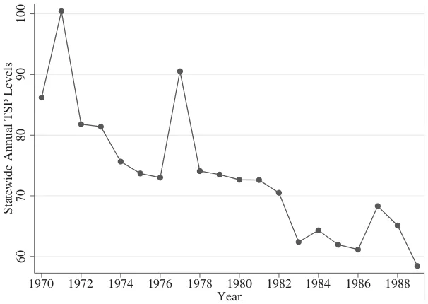
The economy of Texas underwent a sectoral shift as a result of the 1981–83 recession; the manufacturing sector saw decreases in both employment and capacity utilization, and employment shifted to sectors such as retail and services (Orrenius, Saving, and Caputo 2005). This led to a sharp drop in statewide TSPs in a short period of time. Average TSP levels exhibited the greatest changes between 1981– 83, as shown in Figure 2, when state average TSP levels fell by almost 10 micro-grams per cubic meter (µg/m3), a change of approximately 14 percent, and remained permanently lower. This is the largest permanent decrease in Texas in such a short period since the early 1970s.8
Counties with greater shares of their economy in manufacturing saw greater rela-tive decreases in pollution. Almost 50 percent of particulate emissions in 1976 came from industrial production, and the decrease in TSPs during the industrial recession
7. I drop schools with pupil-teacher ratios that are likely “coding errors,” where I call any given year a coding error if that year’s pupil-teacher ratio is at least three times the size of the average of all other years at that school.
8. From 1977 to 1978, the annual TSP mean dropped by approximately 15µg/m3, which is likely
Year
1970 1972 1974 1976 1978 1980 1982 1984 1986 1988
Statewide Annual TSP Levels
60
70
80
90
100
Figure 2
Average Texas Total Suspended Particulates Levels Over Time
Notes: Total suspended particulate level is the annual arithmetic mean using all sensors (covering 30 counties) in the main analysis, and is expressed in micrograms per cubic meter of air. The primary period of analysis is 1981–83. Spike in 1977 is likely attributable to dust storms seen in Texas during that year.
correlated strongly with a decrease in industrial and manufacturing production. By 1985 industry’s contribution to total national particulates was down to approximately 37 percent (Environmental Protection Agency 1985; Chay and Greenstone 2003b). I use this relationship as the basis of my IV analysis, where I use the relative share of county-level employment in manufacturing (manufacturing employment divided by all other employment sources) as an instrument for TSPs.
TSP =g(relative manufacturing employment )
(2) year of birth year of birth
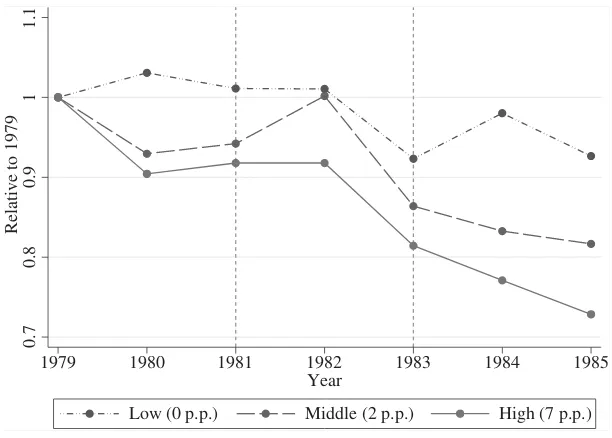
Figure 3 shows how pollution levels changed by changes in manufacturing employ-ment levels. The figure divides counties into terciles based on the absolute change in relative manufacturing employment counties experienced during the recessionary period. Groups with greater decreases in relative manufacturing ended up with greater relative drops in their ambient TSP levels.
Low (0 p.p.) Middle (2 p.p.) High (7 p.p.)
1979 1980 1981 1982
Year
1983 1984 1985
0.7
0.8
0.9
1
1.1
Relative to 1979
Figure 3
Total Suspended Particulate Levels by 1981–83 Change in Relative Manufacturing Notes: Data are the mean total suspended particulate level for a balanced panel of the 30 counties included in the analysis as described in Sections III and V. Values are relative to 1979 levels. Counties are grouped into terciles by absolute change in the primary instrument, annual county-level manufacturing employment divided by all other employment, between 1981 and 1983. Numbers in the legend indicate average per-centage point changes in the instrument for each tercile.
pollution and income are negatively correlated).9 Second, employment data at the county level are available on a yearly basis, so all pollution assignment is on the county by year of birth level. This could be problematic if pollution causes a shift in the timing of birth across years, which would mean the measurement error is correlated with treatment rather than random, and my results must be interpreted with this in mind. Third, the recession may have impacts on test outcomes that are correlated with positive changes in fetal health but not related to pollution. Dehejia and Lleras-Muney (2004) note that babies born in periods of high unemployment are more likely to have better birth outcomes. This could be attributable to maternal behavior modification during recessions or a selection into motherhood effect. This could bias results in the direction of my findings. Finally, the recession and change in county employment makeup could drive migration patterns that could in turn alter the makeup of students taking the test. This change in student composition might
result in changes in test scores that I would incorrectly assign to the impacts of earlier pollution. I now directly address the motherhood selection and migration issues in depth.
A. Selection into motherhood
Dehejia and Lleras-Muney (2004) found much of the improved behavior was driven by selection and behavior of black mothers, who represent a small portion of my sample (approximately 15 percent of all births in the counties used), while white mothers saw a reduction in average health during recessions. In addition, any choice to engage in childbearing behavior must come with a lag. Unfortunately, I do not have the necessary means to directly address the issue of behavior modification, as I have no information about the mothers of the students analyzed. Instead I examine natality records from Texas to see how the composition of mothers may have changed. I consider how TSPs and my instrument are correlated with factors com-monly related to socioeconomic status and child outcomes: maternal age and race, and in what month prenatal care began.10Results are shown in Columns 1 through 4 of Panel A in Table 2. I weight by the number of total live births per county and control for only county and year effects. I find a statistically significant relationship between TSP levels and the share of mothers who are white. This suggests regions with higher pollution have a higher share of white births. The effect is small—a 10-unit difference in TSPs (approximately the change seen during the 1981–83 period) is correlated with a slightly higher probability of a birth being to a white mother (approximately 6 percent of the mean). As an addition consideration I also checked to see if changes in my instrument are correlated with changes in mother effects (Panel B of Table 2), and found no statistically significant effects for mother age or race. There is a correlation between relative manufacturing employment and prenatal usage. Mothers in more manufacturing-intensive counties wait longer to begin pre-natal care. Again, the effects are small, where a 10-unit difference in TSPs is cor-related with a tenth of a month delay.
B. Selective migration
Changes in job composition may have altered the makeup of families via migration patterns. For example, families of poorer performing children move out, or families of higher performing children move in. If those who have worse performing children either (1) moved out of counties that saw greater (lesser) pollution changes as a result of the recession, or (2) were less (more) likely to move in to greater pollution counties after the recession in systematic ways, my results would be biased upward (downward). Note that, if systematic migration were a confounding issue, I expect to see effects in all periods both during and after the recession. If there were sys-tematic differences in the type of child brought in through migration after the
Sanders
837
(1) (2) (3) (4) (5) (6) (7) (8) (9) (10)
Mother Characteristics Student Characteristics
Age Black White Prenatal Male Black Hispanic Asian
Special Education
Economic Distribution
Panel A: Correlation between ambient TSPs and natality and TAAS demographic data
TSP −0.0002 −0.0002 0.0003** 0.0038 0.0002 0.0008** −0.0001 0.0000 0.0004 −0.0004
(0.0037) (0.0001) (0.0001) (0.0041) (0.0004) (0.0004) (0.0006) (0.0003) (0.0005) (0.0005)
Panel B: Correlation between the manufacturing instrument and natality and TAAS demographic data
Instrument 0.0037 −0.0001 0.0001 0.0111*** −0.0013 0.0006 0.0020 −0.0001 −0.0014 0.0000
(0.0052) (0.0004) (0.0003) (0.0039) (0.0010) (0.0005) (0.0013) (0.0005) (0.0018) (0.0008)
cession, that effect should be present in the other, nonrecession periods. I show in Section VI that this is not the case.
A study by the Pew Research Center using American Community Survey data found that Texas has the lowest outward migration rate of the 50 states. 76 percent of the population over age 18 living in the state in 2005–2007 was born there. Texas also ranked low on the inward migration scale (34th out of 50).11Another potential measure of migration is a longitudinal data set that tracks mobility over time, such as the Panel Study of Income Dynamics (PSID). Using PSID data from 2007, ap-proximately 59 percent of 80 responding household heads from Texas indicate they live in the same state in which they grew up (versus the average of 64 percent for all national respondents). Within that same sample, 28 percent of Texas respondents indicated they had not moved at all from 1981 to 2003, (versus 27 percent for all respondents). Jointly, these surveys indicate that mobility within Texas is either on par with or lower than the national average. However, neither addresses the issue of county-level mobility.
As a more concrete analysis of how migration might influence my findings, I consider (1) county-level migration trends across time, and (2) how changes in the student covariates are associated with changes in pollution during year of birth. I use Internal Revenue Service migration data on tax return information to track county-level migration. The benefit of these data is that they cover all individuals that file taxes, including all counties in Texas. The drawback is that data are not available until the 1990–91 tax year. This does, however, show if pollution changes during the recession are correlated with long-run shifts in migration patterns. The average annual outward migration rate varied between 4.9 and 5.8 percent per year, while the annual inward migration rate varied between 4.2 and 6.6 percent. To see how rates varied with pollution changes during the recession, I first calculate the 1981–83 change in pollution for each county. I then regress that change on inbound and outbound migration percentages (the number of migrating individuals, including primary filers and exemptions, divided by the population) for each tax year from 1990 through 2004. Of the resulting regressions, none found statistically significant results. I note that in each case after 1992 the estimated relationship between lution change and migration rates was negative (counties that had the lowest pol-lution changes had greater inward and outward migration rates). Results are omitted for simplicity but are available upon request.
I next consider the statistical association between student covariates and pollution between 1981 and 1983. These results are shown in Columns 5 through 10 in Panel A of Table 2. I run regressions with each of my demographic covariates as an outcome variable, controlling for only school and year of birth fixed effects, and weight by the number of students in each cell. Only the fraction of the school population that is black is significantly correlated with TSPs. A 10-unit difference in TSPs is associated with a 0.8 percentage point decrease in the share of students who are black, or a change of approximately 5 percent. This does suggest potential migration factors, and though I control for race in all regressions, race may be correlated with unobservables and my results should be interpreted with this in mind.
When considering the relationship between student makeup and the instrument (Panel B), I found none to be statistically significant.
In summary, statistically significant correlations exist between some motherhood characteristics and the share of students who are black when considering the 1981– 83 birth cohort. There may be unobservable factors also correlated with pollution that bias OLS regressions. There are no economically significant correlations be-tween my instrument for pollution and any observable mother or student character-istics, and the use of the instrumental variables strategy may alleviate concerns over unobservables.
V. Econometric model
I collapse all student data by demographic group, school of atten-dance, year of birth, and year of test to limit potential omitted variables bias caused by higher levels of aggregation (see Hanushek, Rivkin, and Taylor 1996). I weight all regressions by the number of students in each cell.12The OLS estimation model is:
y =βTSP +α +θ +δX +ωB +ψT +γW +ε ,
(3) s,b,t c,b s b,t s,t c,b c,t c,b s,b,t
where s, c, b, and t refer to school, county, year of birth, and year of the test, respectively. The parameterβis the estimated achievement impact of an additional unit of TSP exposure in the child’s year of birth, αs is a vector of school fixed
effects,θb,tis a vector of year of birth by year of test fixed effects,Xs,tis a vector
of (collapsed individual) school-level student and school covariates,Bc,bis a vector
of economic and demographic covariates in the year of birth, Tc,t is a vector of
economic and demographic covariates in the year of the test, Wc,bis a vector of
county-level weather covariates in the year of birth, andεis an error term. Pollution treatment varies at the county by year of birth level.
In my IV analysis, I model TSPs as a function of all workers in a county employed in the manufacturing industry (SIC code 400) over total county employment levels in all other sectors in a given year. Given a linear relationship where Πis defined as the marginal impact of changes in relative manufacturing employment, the rela-tionship (minus other covariates) is:
manufacturingc,t
TSP =Π ∗100
(4) c,t
allc,t−manufacturingc,t
I multiply the result by 100 to makeΠinterpretable as a percentage change. Clearly, controlling for income is important. The recession was likely accompanied by loss of income, which could in turn have an impact on fetal health and long-run cognitive growth. But income is likely to be correlated with the error term in the regression of pollution on test scores. I instrument for per capita income using changes in
national crude oil prices and the strong link between crude oil prices and income in Texas.13I theorize counties with larger oil extraction sectors prior to the recession had their per capita incomes change more drastically with crude oil prices (similar to the coal reserves and county wages instrument used in Black, Daniel, and Sanders 2002). Due to the limited availability of specific oil extraction employment, I use the more general mining employment (SIC code 200), which contains within it petroleum extraction, drilling, and other oil-mining employment sources. My final income instrument is the annual inflation-adjusted price of crude oil weighted by the fraction of county employment in the mining and extraction industry prior to the recession (using an average of 1976–78 values as the baseline):
miningc,baseline
income =oil price∗
(5) c,t
allc,baseline−miningc,baseline
While annual crude oil price variation occurs on the national level, the instrument varies by county due to the cross-county differences in prerecession mining sector size.
VI. Results
In the discussion that follows, the term “standard deviation” refers to a within-county standard deviation. All regressions control for: student race, eth-nicity, sex, special education, and free lunch status, the school-level pupil/teacher ratio in the year of the exam, income per capita in the year of birth, income per capita in the year of the exam, population density in the year of birth and year of the exam, cubics in temperature, rain, and humidity, and school and year of birth by year of test fixed effects. All standard errors are clustered on county to allow for county-specific correlated errors over time.
Using the 1979–85 cohorts as a whole (Column 1 of Table 3) shows the impact of TSPs is not statistically different from zero. Due to the subtle relationship between pollution and ambient TSPs, the relationship may be undetectable when analyzing mild variations or gradual changes in TSPs driven by long-run trends. Instead I focus on the period of the largest variation, the recession period of 1981–83. This follows Chay and Greenstone (2003b), who exploit a similar methodology to identify the effects of pollution exposure on infant mortality.14I also consider effects by the period just prior and just following the recession period to investigate the presence of trends. Columns 2, 3, and 4 show OLS results for a sample restricted to those born in the periods spanning 1979–81, 1981–83, and 1983–85, respectively (note this causes some overlap in students across samples). The results are statistically
13. Rising oil prices helped Texas partially avoid the earlier stages of the industrial recession, but by 1981, external oil supply increased substantially, leading to a rapid decrease in the real price of oil.
Sanders
841
(1) (2) (3) (4) (5) (6) (7)
79–85 79–81 81–83 83–85 81–83 81–83 81–83
TSP −0.0006 0.0092 −0.0323** −0.0272 −0.0287** −0.0243 −0.0010*
(0.0074) (0.0113) (0.0146) (0.0193) (0.0135) (0.0170) (0.0005)
TSPt + 1 −0.0175* −0.0144
(0.0096) (0.0138)
TSPt + 1 0.0188 0.0215
(0.0127) (0.0149)
TSPt + 2 0.0022
(0.0119)
TSPt + 2 0.0087
(0.0136)
Impact of one Standard DeviationΔin TSP
Δin TLI score 0.00 0.07 −0.24 −0.20 −0.21 −0.18 −0.01
% s.d. in TLI −0.04 0.58 −2.04 −1.72 −1.82 −1.54 −0.06
Observations 73,950 31,895 34,669 30,075 34,669 34,669 34,669
Total students 757,507 322,464 334,956 320,932 334,956 334,956 334,956
insignificant for 1979–81 and 1983–85. For the 1981–83 period the coefficient is statistically significant and has the anticipated negative sign. A standard deviation decrease in average TSPs in the year of birth is associated with 2 percent of a standard deviation increase in eventual test scores. Chay and Greenstone (2003b) note a similar time variation across pre, during, and postrecession periods, and note that the recession period is most useful as “there appears to be greater potential for confounding in cross-sectional analyses and analysis of changes in the surrounding nonrecession years.”
As a further check into the presence of background trends, I repeat the regressions for the 1981–83 period including one year lags and leads of TSPs. Results, shown in Column 5, are robust to the inclusion of both lags and leads, and only the one-year lagged value is marginally significant. This is not in itself problematic. The TAAS data only allow me to identify year of birth, and for some individuals born early in the year the pollution exposure in the prior year is actually the most relevant. Adding two-year lags and leads leaves the coefficient on current TSPs of similar magnitude but increases the standard error enough to remove statistical significance. A joint test of significance on all lags and leads in this specification yields ap-value of 0.27, suggesting they have little explanatory power in this model.
I next consider the impact on the fraction of students passing the standardized exit exams on their first attempt.15Column 7 considers the impact of prenatal pol-lution exposure on the probability of obtaining a passing math score (a TLI score greater than 70) on the first try for the 1981–83 cohort. A standard deviation decrease in ambient pollution in the year of birth is associated with an approximate one percentage point increase in cohort passage rates.
The shock of the recession is unable to overcome the complication of measure-ment error, four types of which may be present. First, true ambient pollution is measured with error at the monitor location. Second, pollution information from air monitors is assigned by using the weighted distance formula as described in Section III. If two counties are similarly located from the same monitors, those two counties will receive similar assignment of pollution levels, thus reducing the variation in county pollution levels beyond its true value. Third, I assign pollution levels to students by assuming the county in which they take the exam is the county in which they were born. Finally, I assign pollution based on year of birth, which introduces noise in the true level of pollution exposure seen by individuals. My instrument can help with the first and second error sources, but unfortunately cannot impact the third or fourth.
OLS may also face omitted variables bias problems. As noted in Section IV, correlations exist between pollution changes and other factors associated with test scores, such as maternal behavior and eventual student demographics. To address such issues, I employ an instrumental variables strategy as discussed in Section V. Using a county-specific manufacturing-based instrument has the additional benefit of a greater level of between-county variation in ambient TSPs, as each county now has a unique source of variation. I report the first-stage coefficients in all IV tables
in addition to the standard statistical significance metrics (discussed below). I use this IV strategy for only the 1981–83 as it is the period of greatest interest given the substantial pollution change, and in the 1979–81 and 1983–85 periods, the first stage is substantially weaker. This suggests that, similar to the subtlety of the effects of pollution on test scores, the relationship between manufacturing production and pollution is harder to discern in the presence of mild changes.
I use limited information maximum likelihood in all estimations due to its greater robustness to weak instruments. In order to assess the strength of the first stage, I report a variety of test statistics. Baum, Schaffer and Stillman (2007) suggest the Kleibergen-Paap F-statistic (Kleibergen and Paap 2006) as a cluster-robust test of overall significance, which I include in my primary tables. I also report the weak-instrument “Angrist-Pischke” multivariate F-test as described in Angrist and Pischke (2009) for both endogenous variables.16Finally, I report thep-value for the Stock-Wright S-statistic as described in Stock and Wright (2000), which tests for joint significance of endogenous regressors in the case of weak-instrument robust infer-ence.
Column 1 of Table 4 shows the primary IV result is statistically significant and approximately 3 times the size of the OLS result. A standard deviation decrease in pollution is associated with almost 6 percent of a standard deviation increase in test scores. The Angrist-Pischke F-values for both endogenous regressors are close to the classic, single endogenous variables F= 10, while the Stock-Wright S-statistic rejects at just above the 3 percent level. Finally, a comparison of the Kleibergen-PaapF-statistic to the Stock-Yogo weak identification critical values as reported in Stock and Yogo (2002) indicates that the instruments fall between the 15 and 20 percent maximal size threshold when using LIML estimation.17 As a whole tests suggest the instruments for both income and manufacturing are well defined. The first-stage coefficient on the manufacturing instrument is approximately 0.61; a one percentage point increase in the ratio of relative manufacturing employment in-creases ambient TSP levels by 0.61µg/m3.18
The larger IV results suggest the presence of downward bias in the OLS estimates. Part of this may be classical measurement error in pollution assignment, though this is unlikely to explain the full difference. The IV estimates identify the local average treatment effect, which may be larger than the average treatment effect identified by OLS. It also suggests the presence of omitted variables bias correlated with pollution and test scores. For example, pollution may be higher in more urban areas where access to prenatal care is greater, which could offset the negative effects of pollution. The treatment of income as endogenous may also be important. There are complex relationships between income and test scores as well as income and pollution, and allowing income to be endogenous may influence results. I address this further below as I explore the robustness of my IV results.
16. I obtain this statistic using the user-written Stata program xtivreg2 (Shaffer 2010).
The
Journal
of
Human
Resources
(1) (2) (3) (4) (5) (6) (7)
Main Adding Additional Exogenous No Income Exogenous TLI
Results Employment Weather Income Control TSP Pass Rate
Panel A: Second-stage impacts
TSP −0.0880*** −0.0649*** −0.0915** −0.1226 −0.0676** −0.0386*** −0.0027**
(0.0311) (0.0223) (0.0421) (0.0745) (0.0328) (0.0129) (0.0012)
Impact of one Standard DeviationΔin TSP
Δin TLI score −0.64 −0.47 −0.67 −0.89 −0.49 −0.28 −0.02
% s.d. in TLI −5.57 −4.11 −5.79 −7.76 −4.27 −2.44 −5.17
Panel B: First-stage results and test statistics
Manf. Ratio 0.0061*** 0.0054** 0.0052** 0.0061*** 0.0044 . 0.0061***
(0.0019) (0.0021) (0.0022) (0.0019) (0.0027) . (0.0019)
Test statistics
TSP AP 17.49 29.02 8.18 2.68 8.27 43.37 17.49
Income AP 25.08 28.64 28.16 . . . 25.08
KPF−statistic 4.34 4.34 2.57 1.19 4.45 33.16 4.34
SWp−value 0.0241 0.0241 0.0170 0.1261 0.2111 0.0279 0.0299
Observations 34,669 34,669 34,669 34,669 34,669 34,669 34,669
Total students 334,956 334,956 334,956 334,956 334,956 334,956 334,956
Column 2 controls for estimated nonmanufacturing employment levels (total county employment minus manufacturing employment divided by population) to test if the first stage is a function of total employment rather than manufacturing em-ployment. The first-stage coefficient is smaller, but second-stage results remain sig-nificant though slightly smaller in magnitude. I next add the number of days in the year of birth that were above 85 degrees and below 25 degrees (given the relation-ship between high temperature and birth weight found in Descheˆnes, Greenstone and Guryan (2009) and the relationship between low temperature and cognitive skills found in Stoecker (2010). I also add the number of days that the average wind speed was above 13 miles per hour, which corresponds to a 4 on the Beaufort scale and is considered fast enough to raise dust on land. Addition of these variables leaves results largely unchanged (Column 3).
Columns 4, and 5, and 6 explore the importance of income per capita in the year of birth in my analysis. In Column 4 I treat only pollution as endogenous while including income per capita as a covariate. This substantially lowers the strength of the first stage by both increasing the standard error and decreasing the coefficient on the manufacturing instrument. The second-stage coefficient on TSPs is now large in magnitude but has ap-value of 0.11. This is a potential concern, particularly if it implies that IV results are driven by the inclusion of the income instrument dis-cussed in Section V. However, this does not appear to be the case. Column 5 repeats Column 4 but excludes income completely. While the estimated impact of TSPs in the second stage is now lower, it remains statistically significant at the 5 percent level. In Column 6, I instrument only for income, leaving TSP as exogenous. Results are smaller than the baseline specification but remain larger than OLS, suggesting potential omitted variables bias in income as well as pollution. As a whole, these findings suggest that how I treat income in the year of birth is an important factor. The IV result is not driven by the inclusion of the income instrument, but failing to treat income as endogenous means both the first and second stage lack clean iden-tification, as income is likely to be correlated with the error term in both states of the regression.
Finally, in Column 7 I return to my main specification but use the TLI passage rate as the outcome variable. Results suggest that a standard deviation decrease in pollution is associated with a three percentage point increase in countywide passage rates, or around 5 percent of a standard deviation.
VII. Discussion
Using standardized test scores as a measure of cognitive development presents some additional complications. TAAS math exam passage rates increased from 57 percent in 1994 to 83 percent in 2002.19 This increase may be due to improved schooling, decreases in ambient pollution levels, or other, less socially productive changes such as “teaching to the test.” In order for these effects to bias results, such practices must vary across counties over time in a manner that is
related with TSPs as well as my instrument, and present during the 1981–83 birth cohorts. The plausibly exogenous nature of the earlier recession shock provides some safeguard against such confounders.
Texas changed how special education students were treated in the 2000 test year. Prior to 2000, special education students did not have their test scores used in the calculation of school-wide passage rates, which were then used to grade schools and determine sanctions. After the 1999–2000 school year, special education scores were included. This could have caused schools/districts to change which populations of students were classified as special education, and the relevant policy change occurs during the testing time frame associated with birth cohorts during the recessionary period.20Richardson (2010) notes that the policy change may have more generally influenced how teachers allocated their time, and caused them to focus on lower achieving students they may have ignored before due to exempt status. In prior drafts I controlled for this more flexibly by allowing the special education effect to vary by year of test, and results were unchanged.
An additional difficulty is the inability to observe parental behavior changes cor-related with the level of treatment. Pollution could have observable impacts such as lowered performance or difficulty concentrating in class, which could in turn cause parents to change the allocation of resources. Almond, Edlund, and Palme (2009) found that, in the case of cognitive damage due to radiation exposure in utero, parental behavior reinforced the effects when considering differences between sib-lings. If this extends to my analysis, it would suggest the effect I find might be partially driven by adjusted parental response.
VIII. Conclusion
I find a statistically significant relationship between prenatal pollution exposure and educational outcomes, specifically performance on standardized high school exit exams. Results are statistically significant only in the periods of the most drastic pollution variation, suggesting a subtle relationship that may be difficult to separate from background trends using minor differences in pollution across counties or gradual changes driven by time. OLS results show a standard deviation decrease in the average annual ambient TSP level during the year of birth is associated with an increase of 2 percent of a standard deviation in test scores, and just under one percentage point increase in countywide test passage rates. Instrumental variables results suggest the same drop in TSPs is associated with an almost 6 percent of a standard deviation increase in test performance and an increase in county passage rates of almost three percentage points. I also address the issues of selection into motherhood and migration.
When gauging the magnitude of such estimates, one must consider the measure-ment of exposure—the average TSP level in the year of birth. The impacts should not be considered the effect of a brief shock (such as, for example, the effect of
pollution on weekly mortality), but rather the impact of an overall lower level of pollution exposure during the entire process of fetal development. As an additional frame of reference, consider the recent finding in Rockoff (2004) that moving one standard deviation up in the distribution of teacher quality raises same-year test scores by approximately 10 percent of a standard deviation. Though the one-time impact of this finding makes it less directly comparable to the long-run effects found with pollution reduction, the magnitudes are nevertheless an interesting comparison. Infants that survive in higher pollution environments may not escape the conse-quences of exposure simply because they avoid becoming low birth weight or mor-tality statistics. Instead, they continue to suffer the effects years later in the form of reduced educational performance. Given that such performance may impact total educational attainment, lifetime earnings, health, and longevity, there are substantial policy implications. For example, Currie and Thomas (2001) find a standard devi-ation increase in test scores is associated with 11–14 percent higher wages and a 3–7 percent higher employment probability at age 33. And if socially marginalized groups are more likely to grow up in polluted environments, pollution exposure may help to partially explain differences in test scores and other long-run outcomes seen across races and socioeconomic groups, and environmental improvement may help to close such gaps. As noted by Reyes (2007), environmental policy and social policy may at times be one and the same.
References
Almond, Douglas and Janet Currie. 2011. “Killing Me Softly: The Fetal Origins Hypothe-sis.”Journal of Economic Perspectives25(3):153–72.
Almond, Douglas, Kenneth Y. Chay, and David S. Lee. 2005. “The Costs of Low Birth Weight.”Quarterly Journal of Economics120(3):1031–83.
Almond, Douglas, Lena Edlund, and Ma˚rten Palme. 2009. “Chernobyl’s Subclinical Legacy: Prenatal Exposure to Radioactive Fallout and School Outcomes in Sweden.”Quarterly Journal of Economics124 (4):1729–72.
Angrist, Joshua D. and Jo¨rn-Steffen Pischke. 2009.Mostly Harmless Econometrics: An Em-piricist’s Companion. Princeton: Princeton University Press.
Barreca, Alan. 2011. “Climate Change, Humidity, and Mortality in the United States.” Jour-nal of Environmental Economics and Management63(1):19–34.
Baum, Christopher F., Mark E. Schaffer, and Steven Stillman. 2007. “Enhanced Routines For Instrumental Variables/Generalized Method of Moments Estimation and Testing.” Stata Journal, 7(4):465–506.
Behrman, Jere R., and Mark R. Rosenzweig. 2004. “Returns to Birthweight.”Review of Economics and Statistics86(2):586–601.
Behrman, Jere R., Mark R. Rosenzweig, and Paul Taubman. 1994. “Endowments and the Allocation of Schooling in the Family and in the Marriage Market: The Twins Experi-ment.”Journal of Political Economy102(6):1131–74.
Black, Dan, Kermit Daniel, and Seth Sanders. 2002. “The Impact of Economic Conditions on Participation In Disability Programs: Evidence from the Coal Boom and Bust.” Ameri-can Economic Review92(1):27–50.
Campbell, A., M. Oldham, A. Becaria, SC Bondy, D. Meacher, C. Sioutas, C. Misra, LB Mendez, and M. Kleinman. 2005. “Particulate Matter in Polluted Air May Increase Bio-markers of Inflammation in Mouse Brain.”Neuro Toxicology26(1):133–40.
Chay, Kenneth Y., and Michael Greenstone. 2003. “Air Quality, Infant Mortality, and the Clean Air Act of 1970.” NBER Working Paper No. 10053.
Chay, Kenneth Y., and Michael Greenstone. 2003. “The Impact of Air Pollution on Infant Mortality: Evidence from Geographic Variation in Pollution Shocks Induced by a Reces-sion.”Quarterly Journal of Economics118(3):1121–67.
Currie, Janet, and Duncan Thomas. 2001. “Early Test Scores, School Quality and SES: Long Run Effects on Wage and Employment Outcomes.”Worker Wellbeing in a Chang-ing Labor Market20:103–32.
Currie, Janet, and Enrico Moretti. 2007. “Biology as destiny? Short-and Long-Run Determi-nants of Intergenerational Transmission of Birth Weight.”Journal of Labor Economics 25(2):231–64.
Currie, Janet, and Matthew Neidell. 2005. “Air Pollution and Infant Health: What Can We Learn From California’s Recent Experience?”Quarterly Journal of Economics 120(3):1003–1030.
Currie, Janet, and Reed Walker. 2011. “Traffic Congestion and Infant Health: Evidence from E-ZPass.”American Economic Journal: Applied Economics3(1):65–90.
Currie, Janet, Eric A. Hanushek, E. Megan Kahn, Matthew Neidell, and Steven G. Rivkin. 2009. “Does Pollution Increase School Absences?”Review of Economics and Statistics 91(4):682– 94.
Currie, Janet, Matthew Neidell, and Johannes F. Schmieder. 2009 “Air Pollution and Infant Health: Lessons from New Jersey.”Journal of Health Economics28(3):688–703. Debes, Frodi, Esben Budtz-Jørgensen, Pal Weihe, Roberta F. White, and Philippe Grandjean,
“Impact of Prenatal Methylmercury Exposure on Neurobehavioral Function at Age 14 Years.”Neurotoxicology and Teratology28(3):363–75.
Dehejia, Rajeev, and Adriana Lleras-Muney. “Booms, Busts, and Babies’ Health.”Quarterly Journal of Economics119(3):1091–1130.
Descheˆnes, Olivier, and Michael Greenstone. 2007. “Climate Change, Mortality, and Adap-tation: Evidence from Annual Fluctuations in Weather in the US,” 2007. NBER Working Paper No. 13178.
Descheˆnes, Olivier, Michael Greenstone, and Jonathan Guryan, “Climate Change and Birth Weight,”American Economic Review: Papers and Proceedings99(2):211–17.
Environmental Protection Agency. 1985. “National Air Quality and Emissions Trends Re-port, 1985.” Washington, D.C.: GPO.
———. 2009. “Integrated Science Assessment for Particulate Matter.” Washington, D.C.: GPO.
Fonken, LK, X. Xu, ZM Weil, G. Chen, Q. Sun, S. Rajagopalan, and RJ Nelson. 2011. “Air Pollution Impairs Cognition, Provokes Depressive-Like Behaviors and Alters Hippocam-pal Cytokine Expression and Morphology.”Molecular Psychiatry.
Friedman, Michael S., Kenneth E. Powell, Lori Hutwagner, LeRoy M. Graham, and W. Gerald Teague. 2001. “Impact of Changes in Transportation and Commuting Behaviors During the 1996 Summer Olympic Games in Atlanta on Air Quality and Childhood Asthma.”Journal of the American Medical Association285(7):897.
Grandjean, Philippe, Pal Weihe, Roberta F. White, and Frodi Debes. 1998. “Cognitive Per-formance of Children Prenatally Exposed to ‘Safe’ Levels of Methylmercury.” Environ-mental Research77(2):165–72.
Hanushek, Eric A., Steven G. Rivkin, and Lori L. Taylor. 1996. “Aggregation and the Esti-mated Effects of School Resources.”Review of Economics and Statistics78(4):611–27. Kleibergen, Frank, and Richard Paap. 2006. “Generalized Reduced Rank Tests Using the
Singular Value Decomposition.”Journal of Econometrics133(1):97–126.
Knittel, Christopher R., Douglas L. Miller, and Nicholas J. Sanders. 2011 “Caution, Drivers! Children Present: Traffic, Pollution, and Infant Health.” NBER Working Paper No. 17222. Lleras-Muney, Adriana. 2010. “The Needs of the Army: Using Compulsory Relocation in
the Military to Estimate the Effect of Air Pollutants on Children’s Health.”Journal of Human Resources45(3):549–90.
Ludwig, Jens, and Douglas L. Miller. 2007. “Does Head Start Improve Children’s Life Chances? Evidence from a Regression Discontinuity Design.”Quarterly Journal of Eco-nomics122(1): 159–208.
Martorell, Francisco. 2004. “Do High School Graduation Exams Matter? A Regression Dis-continuity Approach.” Rand Corporation. Unpublished.
Moretti, Enrico, and Matthew Neidell. 2011. “Pollution, Health, and Avoidance Behavior: Evidence from the Ports of Los Angeles.”Journal of Human Resources46(1):154–75. Neidell, Matthew. 2009. “Information, Avoidance Behavior, and Health: The Effect of
Ozone on Asthma Hospitalizations.”Journal of Human Resources44(2):450 .
———. 2004. “Air Pollution, Health, And Socio-Economic Status: The Effect Of Outdoor Air Quality On Childhood Asthma.”Journal of Health Economics23(6):1209–36. Nilsson, J. Peter. 2009. “The Long-term Effects of Early Childhood Lead Exposure:
Evi-dence from the Phase-out of Leaded Gasoline.” Standford University. Unpublished. Orrenius, Pia M., Jason L. Saving, and Priscilla Caputo. 2005. “Why Did Texas Have a
Jobless Recovery?” Dallas: Federal Reserve Bank of Dallas.
Paul, Annie Murphy. 2010a.Origins: How the Nine Months Before Birth Shape the Rest of Our Lives. Free Press.
Annie Murphy Paul. 2010b. “How the First Nine Months Shape the Rest of Your Life,” Time Magazine, 22 September 2010, adapted from Paul 2010a.
Perera, Frederica P., Zhigang Li, Robin Whyatt, Lori Hoepner, Shuang Wang, David Ca-mann, and Virginia Rauh. 2009. “Prenatal Airborne Polycyclic Aromatic Hydrocarbon Exposure and Child IQ at Age 5 Years.”Pediatrics124(2): e195–e202.
Ponce, Ninez A., Katherine J. Hoggatt, Michelle Wilhelm, and Beate Ritz. 2005 “Preterm Birth: The Interaction Of Traffic-Related Air Pollution with Economic Hardship in Los Angeles Neighborhoods.”American Journal of Epidemiology162(2):140–48.
Raloff, Janet. 2010. “Destination Brain: Inhaled Pollutants May Inflame More than the Lungs.”Science-News177(11).
Reyes, Jessica Wolpaw. 2007. “Environmental Policy as Social Policy? The Impact of Childhood Lead Exposure on Crime.”Berkeley Electronic Journal of Economic Analysis & Policy 7(1):51.
Richardson, Jed T. 2010. “Accountability Incentives and Academic Achievement: The Bene-fit of Setting Standards Low.” Unpublished.
Rockoff, Jonah E. 2004. “The Impact Of Individual Teachers On Student Achievement: Evi-dence From Panel Data.”American Economic Review94(2):247–52.
Sanders, Nicholas J. 2011. “What Doesn’t Kill you Makes you Weaker: Prenatal Pollution Exposure and Educational Outcomes.” SIEPR Discussion Paper 10-019.
Sanders, Nicholas J., and Charles Stoecker. 2011. “Where Have all the Young Men Gone? Using Gender Ratios to Measure the Effect of Pollution on Fetal Death Rates.” NBER Working Paper No. 17434.
Stock, James H., and Jonathan H. Wright. 2000. “GMM with Weak Identification.” Econo-metrica68(5):1055–96.
Stock, James H., and Motohiro Yogo. 2002. “Testing for Weak Instruments in Linear IV Regression.” NBER Technical Working Paper No. 0284.
Stoecker, Charles. 2010. “Chill Out, Mom: The Long Run Impact of Cold Induced Maternal Stress In Utero.” Unpublished.
Suglia, S.F., A. Gryparis, R.O. Wright, J. Schwartz, and R.J. Wright. 2008. “Association of Black Carbon with Cognition Among Children in a Prospective Birth Cohort Study.” American Journal of Epidemiology167(3):280.
Suzuki, Tomoharu, Shigeru Oshio, Mari Iwata, Hisayo Saburi, Takashi Odagiri, Tadashi Udagawa, Isamu Sugawara, Masakazu Umezawa, and Ken Takeda. 2010. “In Utero Ex-posure to A Low Concentration of Diesel Exhaust Affects Spontaneous Locomotor Activ-ity and Monoaminergic System in Male Mice.”Particle and Fibre Toxicology7(1):7. World Bank Group. 1999.Pollution Prevention and Abatement Handboo.The International