Full Terms & Conditions of access and use can be found at
http://www.tandfonline.com/action/journalInformation?journalCode=ubes20
Download by: [Universitas Maritim Raja Ali Haji] Date: 12 January 2016, At: 00:28
Journal of Business & Economic Statistics
ISSN: 0735-0015 (Print) 1537-2707 (Online) Journal homepage: http://www.tandfonline.com/loi/ubes20
Iterated Feasible Generalized Least-Squares
Estimation of Augmented Dynamic Panel Data
Models
Robert F. Phillips
To cite this article: Robert F. Phillips (2010) Iterated Feasible Generalized Least-Squares Estimation of Augmented Dynamic Panel Data Models, Journal of Business & Economic Statistics, 28:3, 410-422, DOI: 10.1198/jbes.2009.08106
To link to this article: http://dx.doi.org/10.1198/jbes.2009.08106
Published online: 01 Jan 2012.
Submit your article to this journal
Article views: 130
Iterated Feasible Generalized Least-Squares
Estimation of Augmented Dynamic
Panel Data Models
Robert F. P
HILLIPSDepartment of Economics, George Washington University, Washington, DC 20052 (rphil@gwu.edu)
This article provides the large sample distribution of the iterated feasible generalized least-squares (IFGLS) estimator of an augmented dynamic panel data model. The regressors in the model include lagged values of the dependent variable and may include other explanatory variables that, while exogenous with respect to the time-varying error component, may be correlated with an unobserved time-invariant compo-nent. The article compares the finite sample properties of the IFGLS estimator to that of GMM estimators using both simulated and real data and finds that the IFGLS estimator compares favorably.
KEY WORDS: Error components; Fixed effects; Generalized method of moments; Linear projection; Quasi maximum likelihood.
1. INTRODUCTION
A well-known and frequently employed model in the litera-ture on panel data methods is the dynamic panel data model. In this model determinants of the dependent variable include both an unobserved time-invariant error component and a lagged value of the dependent variable. As is widely known, the time-invariant error component and the lagged value of the depen-dent variable are correlated, and consequently estimators that are reliable when all of the regressors are strictly exogenous can perform poorly when applied to a dynamic panel data model. For example, applying generalized least squares (GLS) to a dy-namic panel data model will generally produce inconsistent es-timates when only the number of cross sections tends to infinity (Sevestre and Trognon1985).
Blundell and Bond (1998), however, pointed out that apply-ing GLS to an augmented version of the model yields a con-sistent estimator. They derived their augmented model by im-posing an initial condition restriction, and in this sense their analysis is in the tradition of a series of articles that stress the importance of initial conditions for some estimation methods when the time series for each cross section is short (see, e.g., Anderson and Hsiao1981, 1982; Sevestre and Trognon1985; Blundell and Smith1991). In many applications, however, one is less than certain about what initial conditions apply, which suggests that estimation should rely on as few initial condition assumptions as possible.
Moreover, although feasible GLS estimators of Blundell and Bond’s augmented regression are known to be consistent, the asymptotic variance–covariance matrix of such an estimator is currently unknown. Blundell and Bond remarked that the as-ymptotic variance–covariance matrix depends on the distribu-tion of the estimator of the variance–covariance matrix of the errors in the augmented regression (Blundell and Bond1998, p. 129, footnote 12). More specifically, this article shows that the large sample behavior of a two-step feasible GLS estimator depends on the first-round regression estimator it relies upon, which implies we cannot draw any general conclusions about the distribution of two-step feasible GLS estimators of Blun-dell and Bond’s augmented regression.
That conclusion, however, does not apply to iterated feasible GLS (IFGLS). Iterating feasible GLS produces a quasi maxi-mum likelihood (QML) estimate of the augmented model’s pa-rameters, and this article provides the large sample distribution of the QML estimator. Additionally, the article shows that the GLS approach Blundell and Bond proposed applies more gen-erally than their article suggests. For example, it shows that an augmented model follows from moment restrictions without the need for initial condition restrictions like those considered by Blundell and Bond. And, the article generalizes Blundell and Bond’s augmented regression model by allowing forplags of the dependent variable and other explanatory variables that are exogenous with respect to the time-varying error component but may be correlated with the unobserved time-invariant compo-nent. Moreover, using simulated data, the article also compares the IFGLS estimator to GMM estimators in terms of bias and root mean squared error, and finds that the IFLGS estimator compares favorably to the GMM estimators. Experimental re-sults also suggest a normality approximation appears to be more accurate for thet-statistic based on the IFGLS estimator than fort-statistics based on GMM estimators. Finally, the IFGLS and GMM estimators are applied to forecast residential natural gas demand. For this real data application the IFGLS estimator proves to be superior in terms of root mean squared forecast error and mean absolute forecast error.
2. THE MODEL AND AUGMENTED REGRESSION
The model studied in this article is the dynamic unobserved effects model
yi=X1iδ0+X2iβ0+Dτ0+ιTci+ǫi (i=1, . . . ,N).
(1)
Hereyi=(yi1, . . . ,yiT)′,X1iandX2iareT×pandT×K
ma-trices with lagsyi,t−1, . . . ,yi,t−pand explanatory variablesx′itin © 2010American Statistical Association Journal of Business & Economic Statistics July 2010, Vol. 28, No. 3
DOI:10.1198/jbes.2009.08106
410
theirtth rows, respectively,Dis aT×(T−1)matrix with time dummiesdt2, . . . ,dtT in itstth row (heredts=0 or 1 according
ass=tor s=t),ιT is aT×1 vector of ones,ci is an
unob-served time-invariant effect, andǫi=(ǫi1, . . . , ǫiT)′is a vector
of unobserved errors that vary with time and cross section. The explanatory variables inxitare assumed to vary withiand with t(for at least somei) and be strictly exogenous with respect to theǫits, whilecimay have a nonzero mean and may be
corre-lated with some or all of the regressors inxit(t=1, . . . ,T).
Be-cause all of the asymptotic results in this article are established forN→ ∞withT fixed, unobserved time-specific effects are controlled for by the parameter vectorτ0, which is estimated,
while the cross-sectional effect,ci, is taken to be random.
Applying GLS to the model in Equation (1) will gener-ally yield inconsistent estimates whenN→ ∞andT is fixed. Sevestre and Trognon (1985) provided results that shed light on the source of the inconsistency. Their results indicate that, for a simple autoregressive error components model (withβ0=0,
τ0=0, andp=1), the inconsistency of GLS is due to
correla-tion betweenyi0andci(see also Blundell and Bond1998).
Thus, if we can augment the dynamic model in Equa-tion (1) with addiEqua-tional regressors so that the time-invariant component in the new augmented model is uncorrelated with yi0, . . . ,yi,1−p and the elements of X2i, that should
elimi-nate the inconsistency in GLS. To obtain the appropriate aug-mented model, consider the linear projection of ci on 1 and ˜
xi=(x′i1, . . . ,x′iT,yi0, . . . ,yi,1−p)′, which defines linear
projec-tion errors
ai=ci−μ0− ˜xi′θ0 (i=1, . . . ,N), (2)
whereθ0=Var(x˜1)−1Cov(x˜1,c1)andμ0=E(c1)−E(x˜′1)θ0
(cf. Chamberlain1982, 1984). The linear projection relation-shipci=μ0+ ˜xi′θ0+aiholds and theais in Equation (2) are
de-fined, for alli, if the variance–covariance matrix Var(x˜i)and
co-variance matrix Cov(x˜i,ci)are finite, Var(x˜i)is positive definite
(p.d.), and Var(x˜i)−1Cov(x˜i,ci)=θ0andE(ci)−E(x˜′i)θ0=μ0
for alli. [The homogeneity restriction that Var(x˜i)−1Cov(x˜i,ci)
andE(ci)−E(x˜′i)θ0are constant acrossiobviously holds if the
variances and covariances in Var(x˜i) and Cov(x˜i,ci) and the
meansE(ci)andE(x˜i)do not change acrossi.] Equations (1)
and (2) imply the augmented regression:
yi=Wiγ0+ui=Wiγ0+ιTai+ǫi (i=1, . . . ,N), (3)
whereWi is theT×mmatrix[X1i X2i DιT ιTx˜′i] andγ0= (δ′0,β′0,τ′0, μ0,θ′0)′. Now observe that, by augmenting the
re-gressors in Equation (1) with the additional rere-gressors in x˜i,
we get a time-invariant error component ai that is
uncorre-lated with the elements ofx˜i by construction. Thus, although
GLS is inconsistent when applied to Equation (1) because Cov(x˜i,ci)=0, for the augmented model in Equation (3) we
have Cov(x˜i,ai)=0, which suggests GLS should be consistent
when applied to Equation (3).
Before verifying this conjecture, a few comments about how the model in Equation (3) fits within the literature are in or-der. The model in Equation (3) generalizes Blundell and Bond’s (1998) augmented regression. It allows forplags of the depen-dent variable and for arbitrary correlation betweenci and
ele-ments ofxit. Moreover, its derivation relies on weaker
condi-tions than Blundell and Bond exploit. Blundell and Bond made
the initial condition restriction that the conditional mean ofciis
linear inyi0, but this restriction is not required. The augmented
regression in Equation (3) is implied by the linear projection in Equation (2) without any restrictions on the conditional distrib-ution ofci.
Other related articles are Mundlak (1978), Chamberlain (1982, 1984), and Hausman and Kuersteiner (2008). Mundlak (1978) considered a panel data model with exogenous regres-sors, and introduced the idea of augmenting the model with additional regressors to control for correlation between the ex-planatory variables and the unobserved time-invariant effect. Chamberlain (1982, 1984) relied on linear projection arguments and minimum distance estimation methods. And, Hausman and Kuersteiner (2008) used a linear projection to remove time-in-variant effects for feasible GLS estimation of a model in which all of the regressors are exogenous.
Bond and Windmeijer (2002), on the other hand, studied a dynamic model. They exploited a linear projection to estimate a first-order autoregressive panel data model. They augmented the regressoryi,t−1 withyi,1, . . . ,yi,T−1in addition to yi0and
then applied two-stage least squares to their augmented regrsion. They showed that this estimation approach produces es-timates that are numerically identical to a one-step differenced GMM estimator that uses the optimal weight matrix under the assumption of homoscedasticǫits. The sampling performance
of such a one-step differenced GMM estimator is investigated in Section4.
3. GLS, FEASIBLE GLS, AND ITERATED
FEASIBLE GLS
In Section2it was conjectured that GLS applied to the model in Equation (3) should be consistent. To verify this conjecture some conditions are needed. To state these conditions, letei= (ai,ǫ′i)′. For convenience, the conditions are stated for i=1.
The conditions are:
C1: (a) Cov(x˜1,c1)and Var(x˜1)are finite, (b) Var(x˜1)is p.d.,
(c) Cov(ǫ1,x˜1)=0, and (d)e1∼(0,V0)withV0a(T+
1)×(T+1)diagonal matrix having diagonal elements σa02, σǫ20, . . . , σǫ20.
Given C1(a) and C1(b), the linear projection parametersθ0
andμ0are defined. Note that the conditions in C1(a) implicitly
restrict either when the stochastic process generatingy1tbegan
or the parameters inδ0=(δ01, . . . , δ0p)′. To see this, consider
that if the model in Equation (1) describes the behavior ofy1t
for not just t=1, . . . ,T, but also fort=0,−1,−2, . . . ,−s, then for fixed, finite s the moment restrictions in C1(a) can be satisfied without any restrictions on the parameters in δ0.
On the other hand, if we lets→ ∞, then the moment restric-tions in C1(a) require that the parameters inδ0satisfy a
well-known stability condition; specifically, the roots of the equation 1−δ01w−δ02w2− · · · −δ0pwp=0 must lie outside the unit
circle. This is becausex˜1 containsy10, . . . ,y1,1−p, and the
as-sumption that these random variables have finite moments, as in Condition C1(a), relies on the stability properties of the process generating them. Thus, Condition C1(a), and consequently the definitions ofθ0andμ0, rely on either the process generating
412 Journal of Business & Economic Statistics, July 2010
y1thaving begun relatively recently or onδ0satisfying a
stabil-ity condition.
As for the other parts of Condition C1, note that, if C1(c) is satisfied, the restriction thatV0 is diagonal holds if the
ele-ments ofǫ1 are uncorrelated among themselves and with c1.
Also, C1(d) implies the variance–covariance matrix of u1= ιTa1+ǫ1, say 0, has the familiar error-components structured
form of 0=σǫ20IT +σa02JT, whereJT =ιTι′T, andIT is the T×T identity matrix. Furthermore, note that, becauseσǫ20and σa02 are unconditional variances, C1(d) does not rule out con-ditional heteroscedasticity. For example, if E(ǫ1t|x1t)=0 and
var(ǫ1t|x1t)=hǫ(x1t)(t=1, . . . ,T), Condition C1(d) requires E[hǫ(x1t)] =σǫ20 (t=1, . . . ,T), but the latter restriction holds
ifx1tis stationary across time.
The conditions in C1 andT≥p+1 imply moment restric-tions that suggest the consistency of GLS.
Lemma 1. If C1 is satisfied and T ≥p+1, then E(W′1×
−1 0 u1)=0.
All proofs are provided in theAppendix.
The moment restrictionsE(W′1 −01u1)=0suggest that
ap-plying GLS to the regression in Equation (3) will yield a consis-tent estimator ofγ0. The GLS estimator implied by these mo-ment restrictions is, of course,γGLS=(Ni=1W′i −01Wi)−1×
N
i=1W′i − 1
0 yi. This estimator is infeasible because it depends
on the unknown parametersσa02 andσǫ20, but Lemma1also sug-gests a feasible counterpart should be consistent.
In order to define a feasible GLS estimator, observe that
−1
a feasible GLS estimator, based on the first-round estimatorγ˜, can be written asγFGLS=(iN=1W′i (γ˜)−1Wi)−1Ni=1W′i×
(γ˜)−1yi.
Unfortunately, this estimator does not have the same large sample distribution as the GLS estimatorγGLS. If the regres-sors inWiwere all strictly exogenous, then
√
N(γFGLS−γ0) could be expected to have the same asymptotic distribution as √
N(γGLS−γ0)(see, e.g., Prucha1984). However, when lags of the dependent variable appear inWi, the estimation problem
is similar to that considered by Amemiya and Fuller (1967), who showed in a different context that a feasible GLS estimator does not have the same limiting distribution as the GLS esti-mator when lagged endogenous variables appear as regressors (see also Amemiya1985, p. 195). Indeed, Lemma2shows that the large sample behavior of a second-round feasible version of the GLS estimator depends on the large sample behavior of the first-round estimatorγ˜.
To show this result a few more conditions and definitions are needed. Throughout the analysisT is held fixed. Moreover, for the sake of convenience, the simple sampling and moment con-ditions given in Concon-ditions C2 and C3 will be used. Concon-ditions C2 and C3 are:
0 W1)has finite elements, and if Conditions C1 and C2 are
also satisfied,T≥p+1,A0is nonsingular, and
Because the second term on the right-hand side of Equa-tion (6) does not vanish asymptotically, Lemma2reveals that the large sample distribution of a two-step feasible GLS esti-mator is complicated by the dependence of the estiesti-mator on its first-round estimator.
This complication, however, does not arise when feasible GLS is iterated. This follows from the observation that the IFGLS estimator can be interpreted as a QML estimator. To see this, suppose momentarily thatei|˜xi∼N(0,V0)whereV0
is the diagonal matrix defined in C1(d). Then the density of yi given x˜i is (2π )−T/2| 0|−1/2exp[−ui(γ0)′ 0−1ui(γ0)/2].
Using this density and the observations that −01=Q/σǫ20+
JT/(σ02T2) and | 0| =Tσǫ20(T−1)σ02 (Hsiao 1986, p. 38), the
log-likelihood for yi conditional on x˜i can be written as li(γ, σ2, σǫ2)=const− [ln(σ2)+(T−1)ln(σǫ2)+ui(γ)2/σ2+ and so on. In other words, we can iterate feasible GLS to locate a root of the equations
N
i=1
W′i (γ)−1ui(γ)=0, (7)
that is a local maximizer of the concentrated log-likelihood LcN(γ)=LN[γ,σ2(γ),σǫ2(γ)].
That iterating feasible GLS will indeed locate a root of the equations in Equation (7) and a local maximizer ofLNc(·) fol-lows from two facts. The first is thatLcN(γFGLS)≥LN[γFGLS,
σ2(γ˜),σǫ2(γ˜)] ≥LcN(γ˜), and the second is that the second in-equality must be strict ifγFGLS= ˜γ andNi=1W′i (γ˜)−1Wi
is nonsingular, for γFGLS is the unique maximizer of LN[·,
σ2(γ˜),σǫ2(γ˜)]ifNi=1W′i (γ˜)−1Wi is nonsingular. Thus, as
long as the new iterateγFGLSdiffers from the previous iterate, ˜
γ, the iterations are increasing the concentrated log-likelihood. On the other hand, ifNi=1W′i (γ˜)−1Wi is nonsingular and
the iterates converge in the sense that the new fitγFGLS does not differ from the prior fit, i.e.,γFGLS= ˜γ, then a root of the equations in Equation (7) and a local maximizer ofLcN(·)has been found. [Kiefer (1980) made a similar observation for an-other panel data model. Specifically, for a fixed-effects model with exogenous variables and arbitrary intertemporal error co-variances, he noted that feasible GLS applied to a transformed model, when iterated, produces the conditional maximum like-lihood estimate.]
But the fact that iterating feasible GLS will yield a root of the equations in Equation (7) does not guarantee the root is consis-tent. Consistency, indeed, the large sample (N→ ∞, fixedT) distribution of a root of the equations in Equation (7) follows from Conditions C1 through C3 and one additional condition. The additional condition is Condition C4.
C4: H0= −A0+2Tψψ′/(T−1)is negative definite (n.d.).
Ordinarily we can expectA0to be p.d., for this condition is
related toW= [W′1 · · · W′N]′ being full column rank, which
will ordinarily be true. Consequently,−A0can be taken to be
n.d., but this does not guaranteeH0is n.d., for the matrixψψ′
is positive semidefinite. However, Lemma3shows we can de-termine whether or notH0is n.d. by evaluating a scalar.
Lemma 3. SupposeA0is p.d., and letA110 denote the
upper-leftp×pblock ofA−01. Also, letψ1denote thep×1 vector consisting of the firstpelements ofψ [see Equation (4)], and setϑ=2Tψ′1A110 ψ1/(T−1). ThenH0is n.d. if, and only if, ϑ <1.
The parameterϑ can be estimated consistently given a con-sistent estimator ofγ0. Thus we can obtain sample evidence on whether or notϑ <1 (see, e.g., Section4.3).
We can now state the main result of this section. Theorem1 provides the large sample (N→ ∞, fixedT) distribution of a local maximizer ofLcN(·).
Theorem 1. If Condition C3 is satisfied andT≥p+1, then B0=E(S1S′1) has finite elements, and if Conditions C1, C2,
and C4 are also satisfied, then there is a compact subsetŴ⊂ Rm, withγ0in its interior, and a measurable maximizer,γQML, ofLcN(·)inŴsuch that, asN→ ∞(T fixed),
√
N(γQML−γ0)→d N(0,H−01B0H−01).
Note that, because normality is not assumed, the conditions of Theorem1implyγQMLis a QML estimator rather than the maximum likelihood estimator. Also, observe that Theorem1 saysγQML is a local maximizer. Thus the iterations for the
IFGLS estimator should be initialized from a consistent start-ing value.
To better appreciate Theorem1 it is useful to compare the IFGLS or QML estimator to other estimators appearing in the literature. To that end, observe that if ei|˜xi∼N(0,V0) (i=
1, . . . ,N) and (e′i,x˜′i)and(e′j,x˜′j)(i=j) are independent, then
γQML corresponds to a maximum likelihood estimator condi-tional onx˜i(i=1, . . . ,N). Thus the IFGLS estimator is related
to other estimators based on maximum likelihood. Bhargava and Sargan (1983), Blundell and Smith (1991), Blundell and Bond (1998), and Hsiao, Pesaran, and Tahmiscioglu (2002) all discussed maximum likelihood whenp=1. In these articles, initial conditions are a recurring theme. Bhargava and Sargan (1983) and Blundell and Smith (1991) considered various spec-ifications foryi0; in other words, different initial condition
re-strictions are considered, and they stressed the importance of testing such restrictions. Blundell and Bond (1998), on the other hand, made an initial condition assumption in assuming the conditional mean ofciis linear inyi0, and pointed out that
un-der normality the GLS estimator of their augmented regression is a conditional maximum likelihood estimator. But this condi-tional maximum likelihood estimator depends on 0, and thus
is not feasible. (Blundell and Bond considered a two-step fea-sible GLS estimator in their Monte Carlo simulations.) Hsiao, Pesaran, and Tahmiscioglu (2002) studied maximum likelihood after the unobserved time-invariant component is removed by differencing, and they relied on assumptions about how long ago the process started and conditional moment restrictions. Of course, the conclusion of Theorem1likewise relies on assump-tions, but they differ from those used in earlier articles. For example, C1 through C4 allow for stochastic processes gen-erating the yits that began recently or long ago. (However, if
those processes began in the distant past, then, as already noted, the elements ofδ0must satisfy a stability condition.) Also,
al-though the IFGLS estimator has been related to other estimators by thinking of it as a conditional maximum likelihood estima-tor, Theorem 1 does not rely on any conditional distribution assumptions.
4. FINITE SAMPLE BEHAVIOR
4.1 Monte Carlo Designs
In order to assess the finite sample behavior of the IFGLS estimator, Monte Carlo experiments were conducted. Experi-mental designs similar to those used by Hsiao, Pesaran, and Tahmiscioglu (2002) were used, though several modifications were made. Following Hsiao et al., the model foryitused in the
experiments was yit =δ0yi,t−1+β0xit +ci+ǫit (t= −t0+
1, . . . ,T), with yi,−t0 =0 (i=1, . . . ,N). The scalar xit was generated by settingxit=αi+0.01t+ζit (t= −t0, . . . ,T,i=
1, . . . ,N), where theζits in this model were generated
accord-ing to the ARMA(1,1)model ζit=ρ0ζi,t−1+εit+0.5εi,t−1
and εit ∼N(0, σε20) (t = −t0 +1, . . . ,T), with ζi,−t0 =0 (i=1, . . . ,N). Moreover, the αis were constructed as αi =
T
t=−t0εit/T∗+ω1i, whereT∗=t0+1+T, and theω1is were generated as independent standard normal variates. The compo-nentciwas generated asci=Tt=−t0ln|xit|/T∗+ω2i, with the ω2is generated as independent standard normal variates. This
specification forci induces correlation betweenci and thexits
and implies the conditional mean ofciis nonlinear inx˜i.
414 Journal of Business & Economic Statistics, July 2010
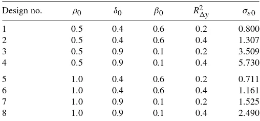
NOTE: The parametersδ0 andβ0 are the regression parameters in the modelyit=
δ0yi,t−1+β0xit+ci+ǫit;ρ0is the autoregression parameter in the ARMA process
erated independently of the xits. The ǫoits were generated as
standardized chi-squared variates, that is, they were constructed as ǫito=(ξ1it2 +ξ2it2 −2)/2, where the ξjits were generated
in-dependently as standard normal variates. The standard devi-ationsd(xit)= [var(αi)+var(ζit)+2 cov(αi, ζit)]1/2 was
cal-In some experiments the heteroscedasticity parameter, q, was set to zero, which produced conditionally homoscedastic ǫits. However, Theorem 1 does not rely on conditional
dis-tribution assumptions. Consequently, it allows for condition-ally heteroscedasticǫits provided they are unconditionally
ho-moscedastic and uncorrelated. Therefore, for some experiments q was set to one, which yielded conditionally heteroscedastic ǫits that were unconditionally homoscedastic.
To investigate the effect, if any, of the starting date, two val-ues for the starting date,−t0, were considered. Some
simula-tions used a recent starting date (t0=1), while others relied
on a starting date in the distant past (t0=50). Moreover, two
sets of values for(N,T)were used in the experiments—(50,5) and(500,5)—and eight different combinations of the parame-tersδ0,β0,ρ0, and σε20 were considered. These combinations
are listed in Table 1. The four combinations with δ0=0.4
were also used by Hsiao, Pesaran, and Tahmiscioglu (2002). For the four combinations withδ0=0.9, I followed Hsiao et
al. in setting σε20 so that the R2 for the differenced equation yit=δ0yi,t−1+β0xit+ǫitwas either 0.2 or 0.4.
4.2 Estimators
For the sake of comparison, in addition to calculating IFGLS estimates, GMM estimates were also calculated. Five GMM es-timators were considered.
Two of these estimators were studied by Arellano and Bond (1991). To define the two estimators Arellano and Bond studied, let y˜ =(△y12, . . . ,△y1T, . . . ,△yN2, . . . ,△yNT)′; let T−1 square matrix with twos running down the main diagonal, minus ones in the first subdiagonals, and zeros everywhere else. Then, a one-step differenced GMM estimator ofb0=(δ0, β0)′
A third GMM estimator studied exploits additional moment restrictions. The estimatorsbGMM1 andbGMM2 are based on
the moment restrictionsE[Z′1iǫ˜i(b0)] =0, but these are not all
of the linear moment restrictions implied by the Monte Carlo designs considered in this article. In particular, weakly exoge-nous xits, and ǫits that are uncorrelated withci, uncorrelated
among themselves, and unconditionally homoscedastic, imply
(see Ahn and Schmidt1995). An asymptotically efficient es-timator based on the moment restrictions E[Z′1iǫ˜i(b0)] =0
Weak instruments are known to exacerbate the finite sam-ple bias of GMM estimators. Thus, two additional GMM es-timators, which excluded weak instruments, were considered. These estimators were the same asbGMM1andbGMM2except
that they excluded the weak instrumentsxi,t+1, . . . ,xiT from the tth diagonal block ofZ1i(t=1, . . . ,T−1).
Finally, in addition to studying the sampling behavior of
bGMM2 =(δGMM2,βGMM2)′, this estimator was used to
ob-tain initial estimates ofδ0 andβ0 for the feasible GLS
itera-tions. To get initial estimates of the linear projection parameters μ0andθ0, ordinary least squares was applied to the equation yit−δGMM2yi,t−1−βGMM2xit=μ0+ ˜x′iθ0+errorit.
4.3 Finite Sample Bias and Efficiency
For each design in Table1, starting valuet0,
heteroscedastic-ity parameter valueq, and sample size, 5,000 independent sam-ples were generated in order to calculate bias and root mean squared error estimates for the IFGLS and GMM estimators ofδ0andβ0. This section provides finite sample bias and root
mean squared error estimates.
Not all of the Monte Carlo results are provided, however. For instance, due to space limitations, the Monte Carlo results for
β0are omitted. The results forβ0can be summarized by noting
that the IFGLS estimator of β0 was always much less biased
than the GMM estimators ofβ0and its root mean squared
er-ror was comparable to that of the best of the GMM estimators (which was not the same GMM estimator for all experiments).
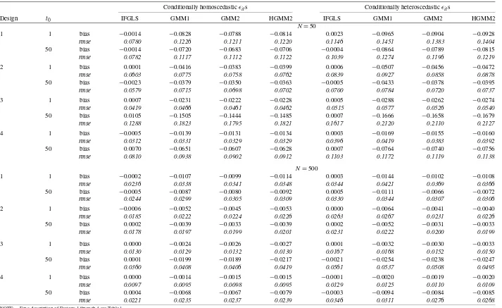
Estimation of δ0 was characterized by greater divergence
in the performance of the IFGLS and GMM estimators. Ta-ble 2 provides bias and root mean squared error estimates for the IFGLS estimator of δ0 and for the first elements of
bGMM1,bGMM2, andbHGMM2 (henceforth, GMM1, GMM2,
and HGMM2). Results for the one-step and two-step GMM es-timators ofδ0that excluded weak instruments are omitted
be-cause excluding weak instruments did not, in general, lead to efficiency improvements. Also, when estimatingδ0, the Monte
Carlo results forρ0=0.5 andρ0=1.0 were similar and,
there-fore, to conserve space, only results forρ0=0.5 are provided.
In other words, the results for Designs 1 through 4 are provided. For all of the experiments, the IFGLS estimator of δ0
ex-hibited little bias, while the bias of the GMM estimators was substantial enough that the GMM estimators often compared poorly to the IFGLS estimator in terms of root mean squared error. For example, for small samples (N=50) the IFLGS esti-mator almost always had the smallest root mean squared error. The small sample superior performance of the IFGLS estima-tor was most pronounced for the designs with conditionally ho-moscedasticǫits. ForN=50 and conditionally homoscedastic ǫits, the IFGLS estimator ofδ0gave, on average, a reduction in
root mean squared error of about 21% compared to the GMM2 estimator’s root mean squared error, and in some cases the re-duction was as much as 30% or more. (ForN=50, GMM2 generally had the smallest root mean squared error among the GMM estimators ofδ0.)
As expected, the bias estimates for the GMM estimators were generally smaller in large samples (N=500) than in small sam-ples. And, as a result, the root mean squared error performance of the GMM estimators ofδ0generally improved relative to the
IFGLS estimator in large samples. But even for large samples, the IFGLS estimator had, in most cases, the smallest root mean squared error when theǫits were conditionally homoscedastic.
In fact, for most of the experiments for whichN=500 and the ǫits were conditionally homoscedastic, the IFGLS estimator of δ0also had the smallest standard deviation. [Standard deviation
estimates can be recovered from the data provided in Table2 by using the relationshipsd=(rmse2−bias2)1/2, wheresd de-notes a standard deviation estimate andrmseis the root mean squared error.]
However, forN=500 and conditionally heteroscedasticǫits,
the bias estimates and standard deviations of the GMM estima-tors were sufficiently small that the IFGLS estimator ofδ0no
longer had the smallest root mean squared error in most cases. Indeed, for the large sample experiments with conditionally het-eroscedasticǫits, the HGMM2 estimator ofδ0usually had the
smallest root mean squared error. For the experiments in which the HGMM2 estimator improved on the IFGLS estimator, the reduction in root mean squared error provided by the HGMM2 estimator was about 13% on average.
Finally, for each sample,ϑ was estimated and the estimate was compared to one in order to obtain sample evidence on the negative definiteness ofH0. In order to estimateϑ, observe that,
forp=1, we haveϑ=2Ta110 (tT=−11φt/T)2/(T−1), wherea110
occupies the first row, first column ofA−01and theφts are
de-fined in Equation (5). The terma110 was estimated with the first row, first column element of(Ni=1W′i (γ˜)−1Wi/N)−1. Here
˜
γ is the starting value for the IFGLS iterations. (This consistent starting value is described at the end of Section4.2.) Theφts
are defined in terms ofδ0[see Equation (5)], and this
parame-ter was estimated with δ˜, the first element of γ˜. ForN=50, 99.49% of the time, the estimate ofϑ was less than one, while forN=500, it was less than one in 99.97% of the samples. [As expected, the Hessian ∂2LcN(·)/∂γ∂γ′ was always n.d. when evaluated at the IFGLS estimate.]
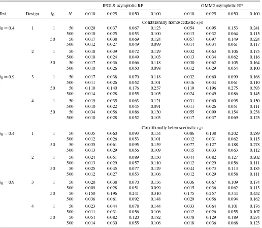
4.4 Hypothesis Tests
To see how useful the asymptotic theory provided in Theo-rem1is for approximating rejection probabilities, Monte Carlo data were also used to evaluate two-tailedt-tests. For Designs 1, 2, 5, and 6 the true null hypothesisδ0=0.4 was tested, while
for Designs 3, 4, 7, and 8 the true nullδ0=0.9 was tested.
Us-ing the standard normal distribution as the reference distribu-tion, rejection probabilities of 0.01, 0.025, 0.05, and 0.10 were considered. For each design in Table 1, starting valuet0,
het-eroscedasticity parameter valueq, and sample size, 5,000 inde-pendent samples were generated in order to estimate actual re-jection probabilitites for a two-tailedt-test based on the IFGLS estimator and its standard error and for two-tailedt-tests based on the GMM estimators and their standard errors.
Standard errors were obtained from estimated variance– covariance matrices. For a one-step GMM estimator robust standard errors were calculated using the formula(X˜′Z1−1×
Z′1X˜)−1X˜′Z1−1A1N−1Z′1X˜(X˜′Z1−1Z′1X˜)−1. For the
two-step GMM estimators, the standard errors were based on Windmeijer’s (2005) finite sample bias corrected variance– covariance estimators. Moreover, the variance–covariance ma-trix for the IFGLS or QML estimator was estimated with HN(γQML)−1BN(γQML)HN(γQML)−1/N, where HN(γ) is
given by Equation (A.5) in the Appendix and BN(γ) =
N
i=1Si(γ)Si(γ)′/N with Si(γ) = W′i (γ)−1ui(γ) + {ui(γ)′Qui(γ)/[σǫ2(γ)(T −1)] −ui(γ)2/σ2(γ)}ψ(δ), where
ψ(δ)is the estimate ofψbased onδ[see Equation (4)]. Table3provides results for conditionally homoscedastic and conditionally heteroscedastic ǫits. Because the results for the
GMM estimators were similar, Table3reports estimated rejec-tion probabilities for only the GMM2 and IFGLS estimators in order to conserve space. Moreover, the results for Designs 5 through 8 were similar to those for Designs 1 through 4, and thus only the latter are provided.
For small samples (N=50), the estimated rejection probabil-ities in Table3 exceed the corresponding asymptotic rejection probabilities. Moreover, conditional heteroscedasticity exacer-bates this tendency to over reject. But the rejection probabilities for thet-test based on the IFGLS estimator are better approxi-mated by the standard normal rejection probabilities than is the case for thet-test based on the GMM estimator.
As expected, for large samples (N=500), the standard nor-mal rejection probabilities provide better approximations to the
416
Jour
nal
of
Business
&
Economic
Statistics
,
July
2010
Table 2. Bias and root mean squared error estimates for IFGLS and GMM estimators ofδ0
Conditionally homoscedasticǫits Conditionally heteroscedasticǫits
Design t0 IFGLS GMM1 GMM2 HGMM2 IFGLS GMM1 GMM2 HGMM2
N=50
1 1 bias −0.0014 −0.0828 −0.0788 −0.0814 0.0023 −0.0965 −0.0904 −0.0928
rmse 0.0780 0.1226 0.1211 0.1220 0.1146 0.1451 0.1383 0.1404
50 bias −0.0014 −0.0720 −0.0683 −0.0706 −0.0004 −0.0864 −0.0789 −0.0815
rmse 0.0782 0.1117 0.1112 0.1122 0.1039 0.1274 0.1196 0.1219
2 1 bias 0.0001 −0.0416 −0.0383 −0.0399 0.0006 −0.0507 −0.0456 −0.0472
rmse 0.0603 0.0775 0.0758 0.0762 0.0839 0.0927 0.0858 0.0878
50 bias −0.0023 −0.0379 −0.0350 −0.0363 −0.0005 −0.0433 −0.0378 −0.0395
rmse 0.0579 0.0715 0.0698 0.0702 0.0700 0.0784 0.0720 0.0737
3 1 bias 0.0007 −0.0231 −0.0222 −0.0228 0.0005 −0.0288 −0.0262 −0.0274
rmse 0.0419 0.0466 0.0461 0.0462 0.0515 0.0577 0.0526 0.0540
50 bias 0.0105 −0.1505 −0.1444 −0.1485 0.0007 −0.1666 −0.1658 −0.1679
rmse 0.1288 0.1823 0.1795 0.1821 0.1617 0.2120 0.2110 0.2127
4 1 bias −0.0005 −0.0139 −0.0131 −0.0134 0.0003 −0.0169 −0.0155 −0.0160
rmse 0.0312 0.0331 0.0329 0.0329 0.0396 0.0419 0.0383 0.0392
50 bias 0.0070 −0.0651 −0.0607 −0.0628 0.0007 −0.0764 −0.0740 −0.0756
rmse 0.0810 0.0938 0.0902 0.0912 0.1103 0.1172 0.1119 0.1138
N=500
1 1 bias −0.0002 −0.0107 −0.0099 −0.0114 0.0003 −0.0144 −0.0102 −0.0108
rmse 0.0236 0.0338 0.0341 0.0348 0.0344 0.0421 0.0369 0.0366
50 bias −0.0005 −0.0087 −0.0080 −0.0092 0.0005 −0.0111 −0.0066 −0.0072
rmse 0.0244 0.0299 0.0305 0.0309 0.0330 0.0344 0.0307 0.0306
2 1 bias −0.0006 −0.0052 −0.0045 −0.0053 0.0000 −0.0064 −0.0041 −0.0040
rmse 0.0185 0.0222 0.0224 0.0226 0.0263 0.0267 0.0231 0.0226
50 bias 0.0002 −0.0039 −0.0033 −0.0039 0.0002 −0.0052 −0.0031 −0.0033
rmse 0.0178 0.0197 0.0199 0.0201 0.0231 0.0222 0.0200 0.0199
3 1 bias 0.0000 −0.0024 −0.0026 −0.0027 0.0001 −0.0032 −0.0030 −0.0033
rmse 0.0130 0.0129 0.0132 0.0130 0.0167 0.0168 0.0152 0.0150
50 bias 0.0001 −0.0199 −0.0189 −0.0217 −0.0021 −0.0254 −0.0238 −0.0247
rmse 0.0360 0.0408 0.0406 0.0419 0.0561 0.0537 0.0508 0.0495
4 1 bias 0.0000 −0.0014 −0.0015 −0.0015 −0.0001 −0.0020 −0.0019 −0.0020
rmse 0.0097 0.0095 0.0098 0.0095 0.0129 0.0125 0.0110 0.0109
50 bias 0.0004 −0.0068 −0.0067 −0.0079 −0.0003 −0.0094 −0.0084 −0.0085
rmse 0.0221 0.0235 0.0237 0.0239 0.0346 0.0311 0.0276 0.0268
NOTE: For a description of Designs 1 through 4 see Table1.
Table 3. Rejection probability (RP) estimates fort-tests based on IFGLS and GMM2 estimators (T=5)
IFGLS asymptotic RP GMM2 asymptotic RP
Test Design t0 N 0.010 0.025 0.050 0.100 0.010 0.025 0.050 0.100
Conditionally homoscedasticǫits
δ0=0.4 1 1 50 0.020 0.037 0.067 0.123 0.054 0.095 0.153 0.241
500 0.010 0.025 0.053 0.100 0.013 0.032 0.064 0.115
50 50 0.017 0.038 0.069 0.124 0.057 0.097 0.149 0.224
500 0.012 0.027 0.049 0.099 0.014 0.034 0.061 0.117
2 1 50 0.018 0.039 0.072 0.129 0.032 0.063 0.106 0.175
500 0.010 0.024 0.049 0.103 0.013 0.034 0.062 0.116
50 50 0.017 0.036 0.066 0.118 0.030 0.062 0.105 0.164
500 0.010 0.026 0.050 0.098 0.012 0.029 0.054 0.100
δ0=0.9 3 1 50 0.017 0.038 0.070 0.118 0.032 0.060 0.099 0.168
500 0.011 0.026 0.052 0.101 0.016 0.034 0.061 0.110
50 50 0.110 0.140 0.176 0.237 0.119 0.196 0.275 0.393
500 0.014 0.028 0.055 0.105 0.024 0.049 0.086 0.145
4 1 50 0.019 0.035 0.063 0.121 0.031 0.060 0.095 0.150
500 0.010 0.022 0.045 0.091 0.011 0.026 0.051 0.111
50 50 0.034 0.056 0.086 0.130 0.055 0.099 0.154 0.238
500 0.010 0.028 0.052 0.103 0.017 0.037 0.069 0.125
Conditionally heteroscedasticǫits
δ0=0.4 1 1 50 0.035 0.060 0.093 0.154 0.086 0.138 0.202 0.289
500 0.012 0.026 0.053 0.101 0.012 0.031 0.062 0.115
50 50 0.035 0.061 0.095 0.159 0.077 0.127 0.188 0.278
500 0.013 0.029 0.056 0.109 0.015 0.033 0.063 0.112
2 1 50 0.024 0.051 0.089 0.150 0.044 0.082 0.127 0.202
500 0.013 0.029 0.057 0.110 0.012 0.029 0.056 0.111
50 50 0.025 0.045 0.077 0.129 0.044 0.073 0.113 0.185
500 0.012 0.027 0.053 0.106 0.012 0.029 0.058 0.111
δ0=0.9 3 1 50 0.020 0.038 0.070 0.136 0.036 0.067 0.109 0.174
500 0.009 0.028 0.051 0.099 0.015 0.036 0.062 0.113
50 50 0.150 0.196 0.241 0.310 0.175 0.257 0.344 0.452
500 0.036 0.061 0.092 0.148 0.029 0.056 0.094 0.162
4 1 50 0.023 0.044 0.078 0.144 0.033 0.064 0.101 0.176
500 0.011 0.031 0.056 0.106 0.012 0.026 0.055 0.107
50 50 0.054 0.082 0.120 0.182 0.078 0.129 0.189 0.274
500 0.014 0.030 0.055 0.106 0.018 0.036 0.068 0.123
NOTE: For a description of Designs 1 through 4 see Table1.
estimated rejection probabilities than for small samples. But still, even for large samples, the asymptotic normality approx-imation is usually more accurate for the t-test based on the IFGLS estimator than for the t-test based on the GMM esti-mator.
Moreover, the data in Table3 illustrate the importance of the stability condition|δ0|<1 when the stochastic processes
generating theyits begin long ago. Consider, for example, the
results for Design 3, a design for whichδ0=0.9. Whent0=1,
the Design 3 results for the IFGLS and GMM2 estimators are comparable to most other cases. However, fort0=50, the
as-ymptotic normality approximations for thet-statistics based on the IFGLS and the GMM2 estimators are quite poor for De-sign 3, especially forN=50. These data indicate that whether or not δ0 is near one can matter when the starting date is in
the distant past, while it is much less important given a recent starting date.
5. A FORECASTING APPLICATION
For a final comparison, IFGLS and GMM were used to fore-cast residential natural gas consumption and the reliability of the forecasts was assessed. The data used were annual ob-servations, from 1987 to 2001, on the amount of natural gas delivered to residential consumers in each of the 48 contigu-ous states in the United States. These data were downloaded from the Energy Information Administration’s Web site (http: // www.eia.doe.gov). Also downloaded were data on the number of residential consumers in each state. From these data, I con-structed natural gas consumption per residence for each state.
The natural gas consumption data were initially modeled with a third-order autoregression with time effects. (This fore-casting model can be derived from a demand-supply model, in which price and lagged values of natural gas consumption ap-pear as explanatory variables, by substituting out price.) How-ever, when the corresponding augmented model was estimated
418 Journal of Business & Economic Statistics, July 2010
with IFGLS over various years, the Wald statistics for testing the joint hypothesis that the coefficients on the second and third lags of the dependent variable are both zero were always in-significant. The model was, therefore, simplified to a first-order autoregressive process with time effects. Specifically, the sim-plified model wasyit=δ0yi,t−1+d′tτ0+ci+ǫit, whereyit
de-notes natural gas consumption per residence in theith state dur-ing thetth year anddt=(dt2, . . . ,dtT)′is a vector of time
dum-mies. This autoregressive model implies the augmented model
yit=μ0+δ0yi,t−1+d′tτ0+θ0yi0+ai+ǫit. (9)
Although the augmented model in Equation (9) can be es-timated directly, the time effects complicate forecasting. The time effects are important for modeling residential consumption of natural gas because much of that consumption is for space heating, and the time effects capture unusually mild or harsh winters. But these effects are contemporaneous with residen-tial gas consumption and are independent across years, mak-ing them unpredictable. Because the purpose of the forecastmak-ing exercise was only to compare IFGLS estimates to GMM es-timates, the time effects were, therefore, eliminated using the transformationy∗it=yit−y·t, wherey·t=
N
i=1yit/N. The
aug-mented model implied by this transformation is
y∗it=δ0y∗i,t−1+θ0y∗i0+a∗i +ǫit∗. (10)
Equations (9) and (10) were both estimated, and the estimates of δ0andθ0 obtained from estimating Equation (10) were
es-sentially the same as the estimates obtained from estimating Equation (9).
For the model in Equation (10), the optimal linear predictor ofy∗i,T+1given the informationY∗i =(yi0∗,y∗′i )′=(y∗i0,y∗i1, . . . , y∗iT)′ isfi,T+1=δ0y∗iT+θ0y∗i0+Y∗′i λ, whereλ=Var(Y∗i)−1×
Cov(Y∗i,a∗i). Furthermore, one can show that Cov(Y∗i,a∗i)= σa2∗φ, whereσa2∗=var(a∗i),φ=(0, φ1, . . . , φT)′,φ1=1, and φj =δ0φj−1+1 (j =2, . . . ,T). Moreover, if we set σǫ2∗ = var(ǫit∗)andσjk=cov(y∗ij,y∗ik)(j=0,1, . . . ,T,k=0,1, . . . ,T),
then one can show by induction that σjj=δ0σj,j−1+θ0σ0j+ φjσa2∗+σǫ2∗ (j=1, . . . ,T),σ0j=δ0σ0,j−1+θ0σ00 (j=1, . . . , T), andσjk=δ0σj,k−1+θ0σ0j+φjσa2∗ (j=1, . . . ,T −1,k= j+1, . . . ,T). Thus, the elements ofλare given in terms of five parameters—δ0,θ0,σ00,σa2∗, andσǫ2∗.
Except forσ00, all of these parameters can be estimated by
applying IFGLS to the regression in Equation (10). In particu-lar, onceγ0=(δ0, θ0)′ is estimated withγQML, thenσǫ2∗ and
σa2∗ can be estimated withσǫ2∗(γQML)=
N
i=1u∗i(γQML)′×
Qu∗i(γQML)/[(T−1)N]andσa2∗(γQML)=Ni=1u∗i(γQML)2/ N−σǫ2∗(γQML)/T, whereu∗i(γ)=ι′Tu∗i(γ)/T,u∗i(γ)=y∗i −
W∗iγ,γ =(δ, θ )′, and thetth row ofW∗i is(y∗i,t
−1,y∗i0)(t=
1, . . . ,T). As for σ00, it was estimated withσ00=Ni=1y∗i02/ (N−1). These estimates were then used to approximate the optimal linear predictorfi,T+1, an approximation referred to in
the sequel as a IFGLS prediction.
To construct an alternative approximation to fi,T+1, the
pa-rameter δ0 in the differenced model y∗it=δ0y∗i,t−1+ǫit∗
was first estimated with a two-step GMM estimator, sayδGMM2.
This estimator relies on the moment restrictionsE[Z∗′1iǫ˜∗i(δ0)] =
0, where ǫ˜∗i(δ) =(ǫ˜i2∗(δ), . . . ,ǫ˜iT∗(δ))′, and ǫ˜it∗(δ) =y∗it − δy∗i,t−1. In other words, it was constructed analogously to the
GMM estimatorbGMM2 described in Section 4.2, except that
the block diagonal elements in the matrixZ∗1i were restricted to y∗i0 in the first block, (y∗i0,y∗i1) in the second block, and (y∗i,t−3,y∗i,t−2,y∗i,t−1)in the remaining blocks (t=3, . . . ,T−1). [DefiningZ∗1iin this manner does not exploit all of the available linear restrictions under the assumption theǫit∗s are uncorrelated acrosst, but when all of the available restrictions were used, the matrixA∗1N=Ni=1Z∗′1iǫ˜∗i(δGMM1)ǫ˜∗i(δGMM1)′Z∗1i became
sin-gular for larger values ofT. This practical constraint on the use of the optimal instrument set was noted by Ziliak (1997).] After δ0was estimated withδGMM2the linear projection parameterθ0
was estimated by regressingy∗it−δGMM2yi∗,t−1ony∗i0. This
es-timate ofθ0and the GMM estimateδGMM2 were then used to
obtain estimates ofσǫ2∗andσa2∗in the same manner the IFGLS estimates were used to obtain estimates of these parameters. For σ00, the estimatorσ00 was again used. Using these estimates
a second approximation tofi,T+1—henceforth referred to as a
GMM2 prediction—was constructed.
Finally, a third approximation to fi,T+1 was constructed.
This approximation was constructed in the same manner as the GMM2 prediction except that, everywhere δGMM2 was
used to construct the GMM2 prediction, another GMM es-timate, sayδHGMM2, was used instead. The GMM estimate
δHGMM2 is based on the moment restrictionsE[Z∗′1iǫ˜∗i(δ0)] =0
andE[Z∗′2iǫ˜∗i(δ0)] =0, where Z∗2i is defined likeZ2i in
Equa-tion (8) except that for the elements ofZ∗2ithe transformedy∗its are used. This last approximation tofi,T+1will be referred to as
a HGMM2 prediction.
Using the data for 1987 to 1995, IFGLS, GMM2, and HGMM2 predictions of 1996 natural gas consumption per res-idence were made for each state. Then the data from 1987 to 1996 were used to construct IFGLS and GMM forecasts of 1997 consumption per residence for each state, and so on, up until consumption for the last year, 2001, was predicted. Thus, for each prediction method, 288 forecasts were constructed: six one-step ahead forecasts for each of 48 states.
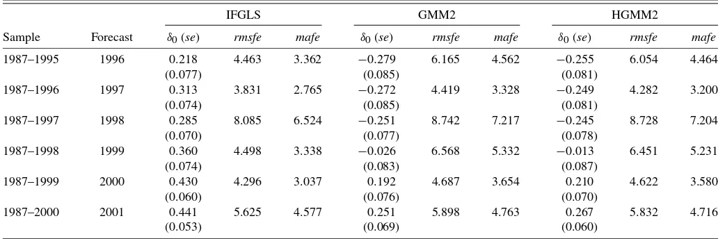
Table4 provides the root mean squared forecast error and mean absolute forecast error for each prediction method and year natural gas consumption was predicted. It also provides the GMM and IFGLS estimates ofδ0used by each prediction
method, along with the standard errors of the estimates. The standard errors of the GMM2 estimates are based on Windmei-jer’s (2005) finite sample bias corrected variance–covariance estimator, as are the standard errors of the HGMM2 estimates.
The GMM estimates ofδ0are always below the IFGLS
esti-mates, a finding consistent with a downward bias in GMM es-timates. Of course, we cannot say which estimates—the GMM or IFGLS—are more accurate, because to do so would require knowledge ofδ0. On the other hand, it is clear which estimates
are preferable for making forecasts, and this suggests some-thing about their reliability. The forecasts based on IFGLS give reductions in root mean squared forecast error and mean ab-solute forecast error ranging from 5%–32% and 4%–37%, re-spectively, compared to forecasts that rely on estimatingδ0via
the GMM2 estimator. The predictions based on the HGMM2 estimator ofδ0 are only marginally better than those based on
the GMM2 estimator. When comparing the IFGLS predictions to the HGMM2 predictions, the IFGLS predictions give reduc-tions in root mean squared forecast error and mean absolute forecast error ranging from 4%–30% and 3%–36%.
Table 4. Forecasting performance of IFGLS and two-step GMM
IFGLS GMM2 HGMM2
Sample Forecast δ0(se) rmsfe mafe δ0(se) rmsfe mafe δ0(se) rmsfe mafe
1987–1995 1996 0.218 4.463 3.362 −0.279 6.165 4.562 −0.255 6.054 4.464
(0.077) (0.085) (0.081)
1987–1996 1997 0.313 3.831 2.765 −0.272 4.419 3.328 −0.249 4.282 3.200
(0.074) (0.085) (0.081)
1987–1997 1998 0.285 8.085 6.524 −0.251 8.742 7.217 −0.245 8.728 7.204
(0.070) (0.077) (0.078)
1987–1998 1999 0.360 4.498 3.338 −0.026 6.568 5.332 −0.013 6.451 5.231
(0.074) (0.083) (0.087)
1987–1999 2000 0.430 4.296 3.037 0.192 4.687 3.654 0.210 4.622 3.580
(0.060) (0.076) (0.070)
1987–2000 2001 0.441 5.625 4.577 0.251 5.898 4.763 0.267 5.832 4.716
(0.053) (0.069) (0.060)
NOTE: This table provides root mean squared forecast error (rmsfe) and mean absolute forecast error (mafe) of forecasts based on estimatingδ0via GMM and IFGLS; also provided are estimates ofδ0and standard errors (se) reported in parentheses.
6. SUMMARY
This article established the asymptotic (N → ∞, fixed T) distribution of the IFGLS estimator of an augmented dynamic panel data model. The regressors in the augmented dynamic panel data model may include several lags of the dependent variable and other explanatory variables that are uncorrelated with the time-varying error components but correlated with the unobserved time-invariant component.
The article also provided Monte Carlo results indicating that IFGLS estimation can provide substantial improvements on lin-ear GMM estimation in terms of root mean squared error. Finite sample bias is to blame. The salient message of the Monte Carlo results is that the IFGLS estimator has negligible finite sample bias. Because GMM estimators can have substantial finite sam-ple bias, the IFGLS estimator can, therefore, be more accurate in terms of root mean squared error even in situations where GMM estimators have smaller sampling variance.
Furthermore, Monte Carlo experiments were used to investi-gate the reliability of hypothesis tests based on IFGLS estima-tion. For the sampling designs considered, rejection probabil-ities based on the standard normal distribution generally pro-vided better approximations to actual rejection probabilities for t-tests based on the IFGLS estimator than for t-tests based on Arellano and Bond’s (1991) two-step GMM estimator.
Finally, in a forecasting application based on real data, the forecasts based on IFGLS were, in terms of root mean squared forecast error and mean absolute forecast error, superior to fore-casts that relied on estimating the autoregression parameter with GMM. Because the forecasting model was the same, while the methods used to estimate it differed, the most obvious ex-planation for the difference in forecasting performance would appear to be the greater accuracy of the IFGLS estimates.
APPENDIX: PROOFS
In this appendix the main result of the article—Theorem1— is established. In the course of proving this result, Lemmas1 and2are also proven. The appendix concludes with a proof of Lemma3.
To simplify the notation,EN(Bi)will be used to denote the
operation of taking an average where the typical term in the av-erage isBi(i=1, . . . ,N), that is,EN(Bi)=Ni=1Bi/N.
More-over, limits are taken withN→ ∞andTheld fixed.
Proof of Theorem1. That B0 andH0 have finite elements
follows from C3 and T ≥p+1. The details that verify this claim are tedious. Interested readers can obtain them from me on request.
Let gN(γ)=EN[W′i (γ)−1ui(γ)]. Also, let Ŵ⊂Rm be a
compact set such that γ0 is in the interior of Ŵ. If there is a measurableγQMLinŴsatisfyinggN(γQML)=0with
probabil-ity (pr.)→1, then, by the usual mean value theorem expansion, we have√N(γQML−γ0)= −H+N√NgN(γ0)+op(1), where
the superscript “+” denotes the Moore–Penrose inverse,HNis
am×mmatrix with (j,k)th element[∂2LNc(γ(j))/∂γj∂γk]/N,
andγ(j)satisfiesγ(j)−γ0 ≤ γQML−γ0(j=1, . . . ,m). It follows that√N(γQML−γ0)→d N(0,H−01B0H−01)ifH0is of
full rank,√NgN(γ0) d
→N(0,B0), andHN→p H0.
The existence of a compact set Ŵ⊂Rm, withγ
0 in its
in-terior, and a measurableγQML inŴsatisfyinggN(γQML)=0
(with pr.→1) is proven in the course of proving LemmasA.1 throughA.5, which follow. These lemmas also establish that √
NgN(γ0) d
→N(0,B0)andHN p
→H0. Thus, they prove
The-orem1.
Lemma A.1. Letui=u′iιT/TandWi=W′iιT/T. If C1 holds,
thenE(W1u1)/σ02= −E(W1′Qǫ1)/σǫ20=ψ forT≥p+1. Proof. Let z1t = (x′1t,dt2, . . . ,dtT,1,x˜′1)′ (t = 1, . . . ,T).
ThenW′1=(y1,−1, . . . ,y1,−p,z′1), wherez1=Tt=1z1t/Tand y1,−j=Tt=1y1,t−j/T (j=1, . . . ,p). Equation (1), C1(a), and
C1(b) imply y1= W1γ0 +ιTa1+ǫ1 with a1 defined by
Equation (2) fori=1; hence,E(z1a1)=0. Also,E(z1ǫ1t)=
0 (t = 1, . . . ,T) by C1(c) and C1(d). Thus, E(W1u1) = (E(y1,−1u1), . . . ,E(y1,−pu1),0′)′. Moreover, E(y1,−ju1) =
0
t=1−jE(y1tu1)/T+Tt=−1jE(y1tu1)/T=0+Tt=−1jE(y1tu1)/ T (j=1, . . . ,p). If C1 is satisfied, then E(y1tu1)=φtσ02 (t=
1, . . . ,T−j) with theφts defined as in Equation (5). Collecting
420 Journal of Business & Economic Statistics, July 2010
Lemma1 follows from LemmaA.1, as the following proof demonstrates. and the elements ofx˜1have finite second order moments. Let σ2(γ)=σ02−2σ02η(γ)′ψ +η(γ)′E(W1W′1)η(γ), σǫ2(γ)= note that the Cauchy–Schwarz inequality and the boundedness ofη(·)′η(·)onŴimply the law of large numbers, and LemmaA.1. This last observation and the fact that the right-hand side of Equation (A.1) does not depend onγreveals thatη(·)′EN(Wiui)
tributed with null mean vectors and finite variance–covariance matrices, and √NEN[ǫ′iQǫiσ02/(T −1)−u2iσǫ20] is normally
distributed with zero mean and finite variance. These observa-tions, Equation (A.2), and LemmaA.2implyϕN=op(1).
To see that √NEN(Si) is multivariate normal
asymptoti-cally, observe thatE(W′1 −01u1)=0(Lemma1) andE{ǫ′1Qǫ1/ [σǫ20(T −1)] −u12/σ02} =0; hence, E(S1)=0. Furthermore,
B0has finite elements. These observations and the Lindeberg–
Levy central limit theorem imply√NEN(Si) d
→N(0,B0).
Using LemmasA.1,A.2, andA.3we can prove Lemma2. Proof of Lemma 2. First, observe that AN
√
+
The second and third terms on the right-hand side of Equa-tion (A.3) →p 0 because √NEN(W′iQǫi/σǫ20+ψ)=Op(1),
Collecting the preceding results gives the conclusion of the lemma.
Lemma A.4. If C1–C4 are satisfied,T≥p+1, then there is a compact subsetŴ⊂Rm such thatγ0 is in the interior ofŴ and there is a measurable maximizer,γQML, ofLcN(·)inŴsuch thatγQML→p γ0.
Proof. By a familiar Taylor series expansion we have
LcN(γ)/N=LcN(γ0)/N+gN(γ0)′η(γ)
Lemmas A.1 through A.3 imply that, upon taking proba-bility limits of the left- and right-sides of Equation (A.4), we have L(γ)=L(γ0)+η(γ)′H(γ∗)η(γ)/2, where γ∗
sat-the only remaining result we need to verify in order to prove Theorem1is thatHN
p →H0.
Lemma A.5. If the conditions of Lemma A.4are satisfied, thenHN
Proof of Lemma3. First it is shown that the conditionsA0is
p.d. andϑ <1 implyH0is n.d. Using a well-known formula
for inverting the sum of two matrices [see, e.g., Henderson and Searle1981, p. 53, equation (3)] and the fact thatψ=(ψ′1,0)′
Now we establish that the conditions A0 is p.d. andH0 is
n.d. implyϑ <1. First, the assumptionH0is n.d. impliesH−01
is defined. This rules outϑ=1 by Equation (A.6). Next,ϑ >1 can be ruled out by establishing a contradiction. Specifically, supposeϑ >1. Setυ=ψ[2T/(T−1)]1/2. For thisυ, we have υ′H−01υ = −ϑ/(1−ϑ ). Butϑ >1 implies−ϑ/(1−ϑ ) >0. Hence,H−01is not n.d. This impliesH0is not n.d., which
con-tradicts the assumptionH0is n.d.
ACKNOWLEDGMENTS
The author thanks two referees and an associate editor for helpful comments on earlier drafts of this article.
[Received May 2005. Revised November 2008.]