Full Terms & Conditions of access and use can be found at
http://www.tandfonline.com/action/journalInformation?journalCode=ubes20
Download by: [Universitas Maritim Raja Ali Haji] Date: 12 January 2016, At: 17:20
Journal of Business & Economic Statistics
ISSN: 0735-0015 (Print) 1537-2707 (Online) Journal homepage: http://www.tandfonline.com/loi/ubes20
Assessing Market Microstructure Effects via
Realized Volatility Measures with an Application to
the Dow Jones Industrial Average Stocks
Basel Awartani, Valentina Corradi & Walter Distaso
To cite this article: Basel Awartani, Valentina Corradi & Walter Distaso (2009) Assessing Market Microstructure Effects via Realized Volatility Measures with an Application to the Dow Jones Industrial Average Stocks, Journal of Business & Economic Statistics, 27:2, 251-265, DOI: 10.1198/jbes.2009.0018
To link to this article: http://dx.doi.org/10.1198/jbes.2009.0018
Published online: 01 Jan 2012.
Submit your article to this journal
Article views: 110
Assessing Market Microstructure Effects via
Realized Volatility Measures with an
Application to the Dow Jones Industrial
Average Stocks
Basel A
WARTANIBusiness School, New York Institute of Technology, Abu Dhabi, United Arab Emirates (UAE) (b.awartani@yahoo.com)
Valentina C
ORRADIDepartment of Economics, University of Warwick, Coventry, UK (v.corradi@warwick.ac.uk)
Walter D
ISTASOImperial College Business School, London, UK (w.distaso@imperial.ac.uk)
Transaction prices of financial assets are contaminated by market microstructure effects. This is partic-ularly relevant when estimating volatility using high frequency data. In this article, we assess statistically the effect of microstructure noise on volatility estimators, and test the hypothesis that its variance is independent of the sampling frequency. We provide evidence based on the Dow Jones Industrial Average stocks. We find that noise has a statistically significant effect on volatility estimators at frequencies of 2–3 min or higher. The independently and identically distributed specification with constant variance seems to be a plausible model for microstructure noise, except for ultra high frequencies.
KEY WORDS: Jumps; Market microstructure; Power variation; Realized volatility.
1. INTRODUCTION
Dating back to Black’s (1986) seminal article, it is a well-accepted fact that transaction data occurring in financial markets are contaminated by market microstructure effects, such as bid-ask spreads, rounding errors resulting from price discreteness and recording errors (see also Hasbrouck 1993; Bai, Russell, and Tiao 2000; Hasbrouck and Seppi 2001; O’Hara 2003; and ref-erences therein). In these articles, it is argued that the observed transaction price can be decomposed into the efficient one plus ‘‘noise’’ because of microstructure effects.
This fact is particularly relevant when dealing with high frequency data, which are often used to compute model-free measures of volatility, such as realized volatility (e.g., see Andersen, Bollerslev, Diebold, and Labys 2001, 2003; Barndorff-Nielsen and Shephard 2002, 2003; Meddahi 2002; Andersen, Bollerslev, and Meddahi 2004) and estimators based on multipower variation (e.g., see Barndorff-Nielsen and Shephard 2004, 2006; Barndorff-Nielsen, Graversen, Jacod, Podolskij, and Shephard 2006; Barndorff-Nielsen, Graversen, Jacod, and Shephard 2006). Although the relevant limit theory suggests that volatility estimates get more precise as the fre-quency of observations increases, this is not necessarily valid in the presence of microstructure noise not accounted for. The effect of microstructure noise on high frequency volatility estimators has been recently analyzed by Bandi and Russell (2006, 2008), Aı¨t-Sahalia, Mykland, and Zhang (2005, 2006), Barndorff-Nielsen, Hansen, Lunde, and Shephard (2008, 2009), Zhang, Mykland, and Aı¨t-Sahalia (2005), Hansen and Lunde (2006), and Zhang (2006). These articles point out that change in transaction prices over very small time intervals are
mainly composed of noise and carry little information about the underlying return volatility. This is because, at least for the class of continuous semimartingale processes, volatility is of the same order of magnitude as the time interval, whereas the microstructure noise has a roughly constant variability. Therefore, as the time interval shrinks to zero, the signal to noise ratio related to the observed transaction prices also tends to zero, and when using standard estimators of volatility one may run the risk of estimating the variance of microstructure noise, rather than the underlying return volatility.
All the articles cited earlier highlight the danger associated with ignoring the presence of noise and acting as if the observed and efficient (latent) prices coincide. They differ, though, when it comes to the prescribed remedies to tackle the problems induced by measurement error. We can distinguish four main approaches in the relevant literature.
1. Use of realized measures robust to the presence of mi-crostructure noise. Consistent volatility estimators were sug-gested by Zhang et al. (2005) and Zhang (2006) for the case of independent noise, and by Barndorff-Nielsen et al. (2005, 2006) and Aı¨t-Sahalia et al. (2006) for the case of dependent noise.
2. Use of the highest frequency at which the microstructure noise effect can be ignored. This approach was followed by Andersen, Bollerslev, Diebold, and Labys (2000), who advo-cated the use of signature plots, where plotting realized volatility
251
2009 American Statistical Association
Journal of Business & Economic Statistics April 2009, Vol. 27, No. 2 DOI 10.1198/jbes.2009.0018
estimators against different sampling frequencies gives a visual idea of the effect of microstructure noise.
3. Assuming a given model for the microstructure error, choose the frequency at which the mean squared error (MSE) is minimized. Bandi and Russell (2005) followed this route and determined the optimal sampling frequency for the case of independent noise.
4. Again, assuming a given model for the microstructure error. By estimating the model describing the noise process, one can construct bias corrected (but inconsistent) measures (e.g., see Oomen 2005; Hansen and Lunde 2006). Andersen, Bollerslev, Diebold, and Ebens (2001), Bollen and Inder (2002), and Hansen, Large, and Lunde (2006) suggested pre-filtering the raw data using moving average models. Although prefiltering does not eliminate the noise, Bandi and Russell (2005) have shown that bias correction of prefiltered data leads to a smaller MSE than bias correction of raw data.
An important question is how to assess empirically the per-formance of the different proposed estimators of volatility in the presence of noise. Bandi and Russell (2008), Andersen, Bollerslev, and Meddahi (2006), Bandi, Russell, and Zhu (2008), Ghysels and Sinko (2006), and Aı¨t-Sahalia and Mancini (2008), studied the relative forecasting ability of various realized vola-tility measures, in terms of a quadratic loss function.
Our article can be associated with the approach outlined earlier in (2). In particular, we contribute to the literature in two directions. First, we provide a test for assessing the impact of market microstructure effects on realized estimators of inte-grated volatility. We do so by comparing two realized vola-tilities computed at different sampling frequencies. Under the null hypothesis of no contamination effect of microstructure noise, the statistic is asymptotically normal; under the alter-native it diverges at an appropriate rate. Generalizing the approach, we choose different sampling frequencies, and run the test comparing realized volatility at a low frequency against the other ones. We then select the highest frequency at which we fail to reject the null hypothesis. Thus, arollingversion of our test can be viewed as a formal counterpart to the signature plots of Andersen et al. (2000). We also provide a version of the test, which is robust to the presence of jumps.
Second, we test the null hypothesis stating that the magni-tude of the error is independent of the chosensampling fre-quency. This hypothesis finds a theoretical justification in Hasbrouck (1993), where the variance of the microstructure error serves as a measure of market quality. In this case, the alternative hypothesis is that the variance of the noise is a function of the time interval between observations. The second test statistic is based on the difference between two estimators of the microstructure noise variance, computed again over different time intervals. Under the null model of an inde-pendently and identically distributed (iid) noise with constant variance, our statistic has a normal limiting distribution, under the alternative it diverges. The null hypothesis here should be interpreted with care. If we fail to reject it, we can conclude that the variance of microstructure noise is constant between the two chosen frequencies. We cannot claim that the magni-tude of the error is independent ofanysampling frequency. In fact, the literature documents that some properties of
micro-structure noise change with the sampling frequency, especially when moving to ultra high frequencies (see Hansen and Lunde 2006); this is also confirmed by our empirical study.
The findings from a Monte Carlo experiment show that the suggested statistics have good finite sample size and power properties. The tests are also applied to transaction data re-corded for the stocks included in the Dow Jones Industrial Average (DJIA), for the period 1997–2002. The empirical analysis sheds some light on the properties of microstructure noise and on the frequencies at which it starts to have a sig-nificant effect on volatility estimators.
The rest of the article is organized as follows. Section 2 describes the methodology and derives the limiting behavior of the two test statistics. Section 3 assesses the finite sample properties of the suggested statistics via a Monte Carlo ex-periment. The empirical findings are reported in Section 4. Section 5 contains some concluding remarks. All the proofs are gathered in the Appendix.
2. METHODOLOGY
2.1 Set-up
We denote the log-price of a generic financial asset, at a continuous timet,asYt.In the article we will assume that the
log-price process belongs to the class of Brownian semi-martingale processes with jumps. We will denote this by writingY2BSMJ. Then:
Yt¼
Z t
0
msdsþ
Z t
0
ssdWsþ
XJt
i¼1
ci; ð1Þ wheremis a predictable drift,sis a cadlag (right continuous with left limit) volatility process, andWis a standard Brownian motion. The jump component is modeled as a sum of nonzero iid random variables,ci, which is independent ofJt and is a finite activity
counting process. Hence, in this article we consider the case of price processes with a finite number of jumps over any fixed time span (see Barndorff-Nielsen and Shephard 2004). On the other hand, the instaneous volatility processs can exhibit inifinitely many jumps, as it is only required to be a cadlag process.
Suppose that we sample the continuous time processYt in
calendar time. We denote the number of daily observations by Tand that of intraday observations byM; therefore, over a fixed time span, sayT, we have a total ofMTobservations. Realized volatility is defined as
RVt;T;M ¼
XMT
i¼1
Ytþi
MYtþiM1
2
; 0#t #TT:
IfYtbelongs to the class of continuous semimartingales (ifJt[
0 "t, i.e., there are no jumps in the log-price process), then (e.g., see Karatzsas and Shreve 1991, Chap. 1), asM!‘,
RVt;T;M !
p Z tþT t
s2sds¼IVt;T: ð2Þ
However, if Yt is the sum of a continuous semimartingale
component and a jump component, then the statement in (2) does no longer hold and (e.g., see Protter 1990),
RVt;T;M !
Barndorff-Nielsen and Shephard (2004) have suggested esti-mators of integrated volatility, based on summing the power of absolute contiguous intraday returns, which are consistent and are robust to the presence of rare and large jumps. In the article, we use tripower variation, given by
TVt;T;M ¼j2=33
k> 0 andSNdenote a standard normal random variable. Now, suppose that transaction data are contaminated by a measurement error, such that
Xtþi
Thus, the observed transaction price can be decomposed into efficient price and ‘‘noise,’’ capturing generic microstructure effects. By simple algebra
XMT
If Yt is a continuous semimartingale, then the first term on
the right of (5) converges in probability to the integrated volatility process. However, if etþi/M is iid and has a
non-zero variance, then the second term diverges as M ! ‘. Of course, if the microstructure noise has a non trivial autocorre-lation structure, the bias implied by the second term in (5) need not diverge at a linear rate (e.g., see Hansen and Lunde 2006). Also, as pointed out by Oomen (2006), the behavior of the bias depends on the sampling schemes (e.g., calendar versus business time). It is easy to see that the last term on the right of (5) is of smaller order than the second term. Thus, allowing for possible correlation between microstructure noise and price will not affect the validity of any asymptotic result. This is important, because the component of noise associated with market infor-mation is generally correlated with the price.
2.2 Assessing the Effects of Microstructure Noise
We assume that the true asset log-price process is generated as in (1). Define the following hypotheses:
H0:E etþi
Thus, our objective is to suggest a procedure to assess whether market microstructure noise has a statistically sig-nificant impact on realized estimators of integrated volatility, at a given sampling frequency.
To test H0versus HA, we propose the following statistic
ZM;N;T;t ¼
is the scaled realized quarticity. The numerator in (8) can be expanded as Inspection of (9) reveals the logic behind the choice of the test statistic in (8); if microstructure noise (under the maintained assumption of no jumps) does not affect realized volatilities at the chosen frequencies, then bothRVt;T;M andRVt;T;N converge
in probability to integrated volatility. Also, by the results of Jacod (1994) and Jacod and Protter (1998),
RVt;T;M
Therefore, under the null hypothesis, provided that as N, M!‘,N/M!0,
This means that the limiting distribution of the test statistic is driven by
which is asymptotically standard normal. Under the alternative, we expect RVt;T;M to be of a larger order of magnitude (in
probability) than RVt;T;N , and so we expect the statistic to
diverge.
In principle, the statistic in (8) can be generalized by using three or more sampling frequencies and then constructing a quadratic form. Suppose, for example, that we have three
sampling frequencies, sayM,N,H, whereN/M!0,N/H!0, andH/M!0. Consider the following statistic
ffiffiffiffiffiffiffi
and note that the covariance between the two preceding terms is asymptotically zero asN/H!0. Thus, under H0, the statistic in (10) is asymptotically distributed as ax22. We leave the issue of power comparison between (10) and (8) to future research. A possible problem with the statistics in (8) and (10) is that standard normal critical values are no longer correct in the presence of jumps, by lack of consistency of realized volatility. Therefore, we also suggest a statistic robust to jumps
ZTM;N;T;t ¼
is the scaled realized quadpower variation, and
a¼j
2.2.1 An Alternative Test. An alternative approach to testing for the hypothesis in (6) is based on the autocorrelation structure of the return process. In fact, if the drift is zero and there is no leverage, then Xtþiþ1
M XtþMi
is a martingale dif-ference process, whereas in the presence of drift and or lever-age, it is asymptotically uncorrelated. Consider the statistic
ACM;T;t ¼
and note that the numerator can be decomposed as
ffiffiffiffiffiffiffiffi
Now, under the null, the last three terms on the right of (14) converge to zero, almost surely, whereas the first term is asymptotically normal with asymptotic variance equal to
RtþT
t s
4
sds:On the other hand, under the alternative,
PMT1
i¼1 e2tþi=Mis the dominant term, so that the statistic diverges to minus infinity. The denominator is a robust estimator of inte-grated quarticity under the null and diverges at a slower rate than the numerator under the alternative, thus ensuring asymptotic unit power.
A limitation of the statistic suggested in (13) is that, in the presence of jumps, it still has a normal limiting distribution, but with an unknown nonzero mean.
2.3 A Specification Test for Microstructure Noise
In this subsection, we derive a test for the hypothesis that microstructure noise has constant variance, independent of the chosensampling frequencies. Failure to reject the model with constant noise variance has important implications for the pur-pose of volatility estimation. First, all the robust estimators pro-posed in the literature, whether based on subsampling methods or on kernel functions or simply on bias correction, rely on the validity of that assumption. Second, important implications for choosing the ‘‘optimal’’ sampling frequency for estimating inte-grated variance using realized volatility are derived assuming the additive model with constant noise variance. Define
Eðetþi=Metþði1Þ=MÞ
The null and alternative hypotheses can be formulated as follows:
H00:nt;M¼nt;N; ð16Þ
and
H0A :nt;M6¼nt;N; forM>N: ð17Þ The null hypothesis tested here is that the variance of the microstructure noise is the same regardless of whether data are recorded at frequency 1/Mor 1/N. The alternative hypothesis is compatible with the diffusion with measurement error model of Gloter and Jacod (2001a,b). As a consequence, the bias may grow less than linearly in the number of intraday observations. The alternative hypothesis is also consistent with the pres-ence of autocorrelation in microstructure noise. In fact, Hansen and Lunde (2006, Corollary 3) showed that in the presence of autocorrelated errors, the bias may be either finite or grow at a rate slower than M. In this sense, the rejection of the null hypothesis can be more broadly interpreted as rejection of the null of iid microstructure noise with constant variance.
We propose the following test statistic
VM;N;L;T;t ¼
whereL is a lower frequency (e.g., 20 min), at which micro-structure noise can be safely ignored. The logic behind the statistic proposed previously is the following. Under the null hypothesis, both RVt;T;M RVt;T;L
=2MT and RVt;T;N
RVt;T;L Þ=2NTconverge to the same probability limit, say nt,
though the former converges faster than the latter. Thus,
ffiffiffiffiffiffiffi
is asymptotically negligible and the statistic in (18) is asymp-totically equivalent to
which has a standard normal limiting distribution (see Theorem A1 in Zhang et al. 2005).
nt,N, and thus the statistic diverges.
The reason why we include the extra term RVt;T;L in the
construction of our test statistic is that, for some sampling frequencies, IVT=MT and IVT=NT may not be negligible.
Carlo investigation confirms that the chosen version of the test performs much better than the unmodified counterpart.
2.4 Main Theoretical Results
In the sequel, we need the following assumptions
A1.Ytis generated as in (1).
A2.RttþTs4
sds<‘;almost surely, for anytandT A3. Eðetþi=Metþði1Þ=MÞ4 <‘;for alltandi A4. There exists ane> 0, such that almost surely
lim inf
A5.etþi/Midentically and independently distributed.
Table 1. Actual sizes of the tests based onZM;N;T;tand
M¼1,440 0.052 0.101 0.051 0.103
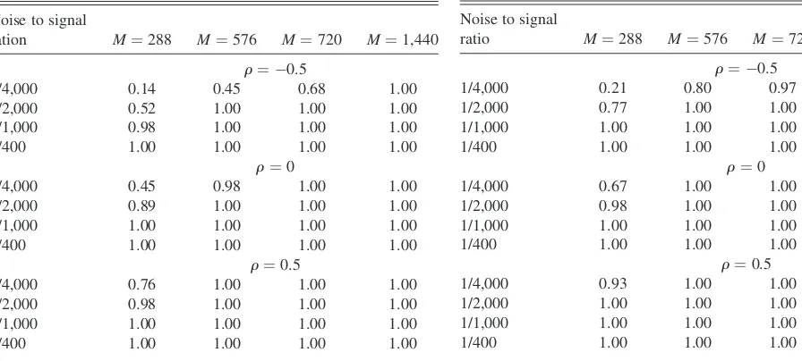
Table 2. Size-adjusted power of the test based onZM;N;T;tforN¼144,
different values of noise to signal ratios,randM, at the 5% level
Noise to signal
ration M¼288 M¼576 M¼720 M¼1,440
r¼ 0.5
1/4,000 0.14 0.45 0.68 1.00
1/2,000 0.52 1.00 1.00 1.00
1/1,000 0.98 1.00 1.00 1.00
1/400 1.00 1.00 1.00 1.00
r¼0
1/4,000 0.45 0.98 1.00 1.00
1/2,000 0.89 1.00 1.00 1.00
1/1,000 1.00 1.00 1.00 1.00
1/400 1.00 1.00 1.00 1.00
r¼0.5
1/4,000 0.76 1.00 1.00 1.00
1/2,000 0.98 1.00 1.00 1.00
1/1,000 1.00 1.00 1.00 1.00
1/400 1.00 1.00 1.00 1.00
Table 3. Actual sizes of the tests based onACM;T;tfor
different values ofM
5% nominal size 10% nominal size
M¼288 0.051 0.098
M¼576 0.066 0.118
M¼720 0.056 0.106
M¼1,440 0.060 0.109
Table 4. Size-adjusted power of the test based onACM;T;tfor different
values of noise to signal ratios,randM, at the 5% level
Noise to signal
ratio M¼288 M¼576 M¼720 M¼1,440
r¼ 0.5
1/4,000 0.21 0.80 0.97 1.00
1/2,000 0.77 1.00 1.00 1.00
1/1,000 1.00 1.00 1.00 1.00
1/400 1.00 1.00 1.00 1.00
r¼0
1/4,000 0.67 1.00 1.00 1.00
1/2,000 0.98 1.00 1.00 1.00
1/1,000 1.00 1.00 1.00 1.00
1/400 1.00 1.00 1.00 1.00
r¼0.5
1/4,000 0.93 1.00 1.00 1.00
1/2,000 1.00 1.00 1.00 1.00
1/1,000 1.00 1.00 1.00 1.00
1/400 1.00 1.00 1.00 1.00
Notice that A1 and A2 are customary in the literature on realized volatility; A3 requires a finite fourth moment of the market microstructure noise and seems to be trivially satisfied. A4, which is required only under the alternative, is always satisfied providedbM1 andbN1 approach zero at a rate slower than M1 andN1, respectively. In other words, for a given number of intradaily observationsM, we require that under the alternative the variance of the microstructure noise is bounded below by 1/bM, wherebMis a sequence approaching infinity at
a rate slower thanM. Assumption A5 ensures that the estimator used in the denominator of (18) is consistent for the ‘‘true’’ variance. In fact, A5 is required only in Proposition 4. It is worthwhile to point out that assumptions A1–A4 allow for
possible autocorrelation in the noise process and for correlation between the noise and the price process.
Proposition 1.
(1) Let A1 and A2 hold and assume that Jt ¼0 for all t.
Under H0, defined in (6), asM, N!‘, andN/M!0, ZM;N;T;t !
d
Nð0;1Þ:
(2) Let A1–A4 hold. Under HA, defined in (7), asM, N!‘,
fore> 0, lim
M;N!‘Pr ffiffiffi
N
p
b1
N Mb1
MNbN1
ZM;N;T;t >e
¼1:
Proposition 2.
(1) Let A1 and A2 hold. Under H0, defined in (6), asM, N!‘, andN/M!0,
ZTM;N;T;t !
d
Nð0;1Þ:
(2) Let A1–A4 hold. Under HA, defined in (7), asM, N!‘,
fore> 0, lim
M;N!‘Pr ffiffiffi
N
p
b1
N Mb1
MNb
1
N
ZTM;N;T;t >e
¼1:
Proposition 3.
(1) Let A1 and A2 hold and assume thatJt¼0 for allt.Under
H0, defined in (6), asM!‘, ACM;T;t !
d
Nð0;1Þ
(2) Let A1–A4 hold. Under HA, defined in (7), asM!‘,
fore> 0,
lim
M!‘Pr
1
ffiffiffiffiffiffiffiffiffiffi
MbM
p ACM;T;t < e
¼1:
The properties of the specification test for microstructure noise are given in the next Proposition.
Proposition 4.
(1) Let A1–A3 and A5 hold. Under H00;defined in (16), as M, N, L!‘,N/M!0,L/N!0,
VM;N;L;T;t !
d
Nð0;1Þ.
(2) Let A1–A3 hold. Under HA, defined in (17), asM, N,
L!‘, fore> 0, lim
M;N;L!‘Pr
1 ffiffiffiffiffi
NT
p VM;N;L;T;t
>e
¼1:
3. A SIMULATION EXERCISE
In this section, the small sample performance of the pro-posed tests is assessed through a Monte Carlo experiment. We generate log-returns using the simple model
dYt ¼hdWt:
The parameterh¼pffiffiffiffiffiffiffiffiffiffiffiffiffiffi0:0015 has been calibrated to produce a daily integrated volatility equal to the annual average of the Intel stock for 2000 (using realized volatilities at the 5 min frequency). We first simulate a discretized version of the continuous tra-jectory ofYtunder (19), using an Euler scheme. To get a precise
approximation to the continuous path, we choose a very small time interval between successive observations (1/5,760); more-over, the initial value is drawn from the marginal distribution of Yt.We then sample the simulated process at two different
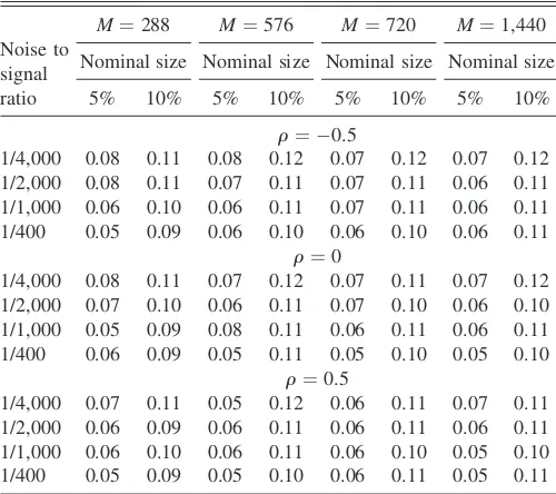
fre-quencies, 1/Nand 1/M, and compute the different test statistics. Table 5. Actual size of the unconditional test based on
VM;N;L;T;tforN¼144,L¼72, different values of noise
to signal ratios,randM
Noise to signal ratio
M¼288 M¼576 M¼720 M¼1,440
Nominal size Nominal size Nominal size Nominal size
5% 10% 5% 10% 5% 10% 5% 10%
r¼ 0.5
1/4,000 0.06 0.10 0.07 0.12 0.08 0.12 0.07 0.11 1/2,000 0.06 0.10 0.07 0.11 0.07 0.11 0.06 0.11 1/1,000 0.06 0.11 0.07 0.11 0.06 0.11 0.06 0.10 1/400 0.05 0.09 0.06 0.11 0.06 0.10 0.05 0.11
r¼0
1/4,000 0.07 0.10 0.06 0.11 0.07 0.11 0.06 0.12 1/2,000 0.06 0.10 0.06 0.11 0.06 0.10 0.06 0.10 1/1,000 0.06 0.10 0.07 0.11 0.05 0.11 0.07 0.11 1/400 0.04 0.09 0.05 0.10 0.05 0.11 0.05 0.11
r¼0.5
1/4,000 0.05 0.10 0.06 0.12 0.06 0.11 0.07 0.13 1/2,000 0.06 0.09 0.06 0.11 0.07 0.11 0.06 0.11 1/1,000 0.06 0.10 0.06 0.12 0.06 0.10 0.05 0.11 1/400 0.05 0.09 0.05 0.10 0.05 0.11 0.05 0.10
Table 6. Actual size of the test based onVM;N;L;T;tforN¼144,
L¼72, different values of noise to signal ratios,randM
Noise to signal ratio
M¼288 M¼576 M¼720 M¼1,440
Nominal size Nominal size Nominal size Nominal size
5% 10% 5% 10% 5% 10% 5% 10%
r¼ 0.5
1/4,000 0.08 0.11 0.08 0.12 0.07 0.12 0.07 0.12 1/2,000 0.08 0.11 0.07 0.11 0.07 0.11 0.06 0.11 1/1,000 0.06 0.10 0.06 0.11 0.07 0.11 0.06 0.11 1/400 0.05 0.09 0.06 0.10 0.06 0.10 0.06 0.11
r¼0
1/4,000 0.08 0.11 0.07 0.12 0.07 0.11 0.07 0.12 1/2,000 0.07 0.10 0.06 0.11 0.07 0.10 0.06 0.10 1/1,000 0.05 0.09 0.08 0.11 0.06 0.11 0.06 0.11 1/400 0.06 0.09 0.05 0.11 0.05 0.10 0.05 0.10
r¼0.5
1/4,000 0.07 0.11 0.05 0.12 0.06 0.11 0.07 0.11 1/2,000 0.06 0.09 0.06 0.11 0.06 0.11 0.06 0.11 1/1,000 0.06 0.10 0.06 0.11 0.06 0.10 0.05 0.10 1/400 0.05 0.09 0.05 0.10 0.06 0.11 0.05 0.11
NOTE: The test is computed conditional on rejecting H0usingZM;N;T;tat the 5% level.
To be consistent with the empirical exercise, we have set
T¼5: In the case of no jumps, we have computed the test statisticZM;N;T;t andZTM;N;T;t forN¼144 andM¼(288, 576,
720, 1,440). Assuming that market is continuously open, the values ofMrange from 5 min to 1 min data; we perform 10,000 replications.
ForZTM;N;T;t ; the jump component has been added to the
continuous price process following Barndorff-Nielsen, and Shephard (2004). In particular, 10 randomly scattered jumps have been added to the log-price process, and the jumps are IN (0,0.64E(IVt)). Therefore, when there is a jump, the jump
component has 64% of the variance as that expected over a day with no jumps.
Results on the empirical sizes of the tests based onZM;N;T;t
andZTM;N;T;t are reported in Table 1. In general, the tests have
good size properties; the test based onZM;N;T;t is a bit
under-sized for M¼288, but asMincreases its empirical size gets closer to the nominal one. The test based onZTM;N;T;t seems to
have slightly better size properties than its counterpart based on realized volatilities.
The power of the statisticZM;N;T;t has been calculated adding
some noise to the data generating process considered pre-viously. In particular, the price process has been simulated for different variances of the microstructure noise, using the noise to signal ratios implied by Bandi and Russell (2007). Also, the cases where the noise is negatively correlated, uncorrelated, and positively correlated with the price process have been considered separately (with r denoting the correlation coef-ficient). The test has good power properties, as can be seen by inspection of Table 2, with the power monotonically increasing in the variance of the microstructure error. The power is also increasing in the correlation coefficientr(the power of the test
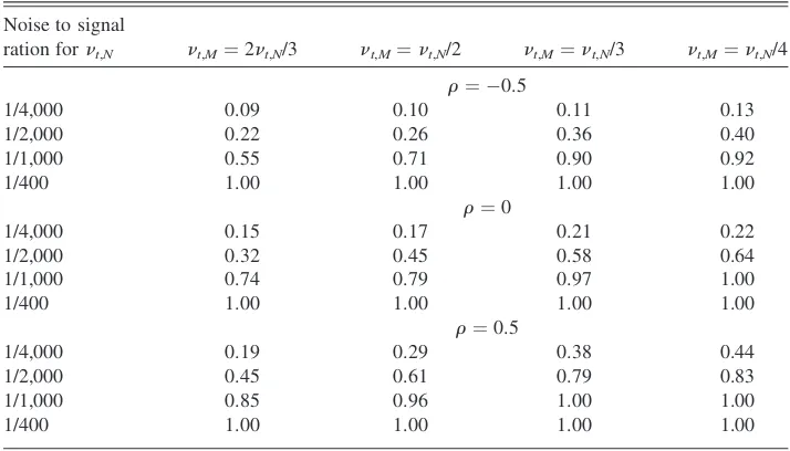
Table 8. Power of the unconditional test based onVM;N;L;T;tforM¼288,N¼144,L¼72,
different values ofnt,Mnt,N, at the 5% level
Noise to signal
ration fornt,N nt,M¼2nt,N/3 nt,M¼nt,N/2 nt,M¼nt,N/3 nt,M¼nt,N/4
r¼ 0.5
1/4,000 0.09 0.10 0.11 0.13
1/2,000 0.22 0.26 0.36 0.40
1/1,000 0.55 0.71 0.90 0.92
1/400 1.00 1.00 1.00 1.00
r¼0
1/4,000 0.15 0.17 0.21 0.22
1/2,000 0.32 0.45 0.58 0.64
1/1,000 0.74 0.79 0.97 1.00
1/400 1.00 1.00 1.00 1.00
r¼0.5
1/4,000 0.19 0.29 0.38 0.44
1/2,000 0.45 0.61 0.79 0.83
1/1,000 0.85 0.96 1.00 1.00
1/400 1.00 1.00 1.00 1.00
Table 7. Power of the unconditional test based onVM;N;L;T;tforN¼144,L¼72, different
values ofM,nt,Mnt,N, at the 5% level
Noise to signal ratio fornt,N
M¼216,
nt,M¼2nt,N/3
M¼288,
nt,M¼nt,N/2
M¼432,
nt,M¼nt,N/3
M¼576,
nt,M¼nt,N/4
r¼ 0.5
1/4,000 0.08 0.10 0.14 0.17
1/2,000 0.18 0.26 0.37 0.39
1/1,000 0.51 0.71 0.90 0.92
1/400 0.96 1.00 1.00 1.00
r¼0
1/4,000 0.12 0.17 0.25 0.28
1/2,000 0.27 0.45 0.58 0.64
1/1,000 0.64 0.79 0.96 0.99
1/400 0.98 1.00 1.00 1.00
r¼0.5
1/4,000 0.18 0.29 0.42 0.44
1/2,000 0.35 0.61 0.76 0.85
1/1,000 0.74 0.96 1.00 1.00
1/400 1.00 1.00 1.00 1.00
based on ZTM;N;T;t displays a qualitatively very similar result
and therefore is omitted for space reasons).
Results for size and power of the test based on ACM;T;t are
reported, respectively, in Tables 3 and 4. The size properties of the test are very good, being really close to the nominal ones, for all the sample sizes considered. Moving to Table 4, the test based onACM;T;t displays higher power than the one based on
ZM;N;T;t : A comparison between the two tests is not possible,
because under the alternative hypothesisACM;T;t :will diverge
at the rate ffiffiffiffiffiffiffiffiffiffiMbM
p
; and ZM;N;T;t will diverge at the rate
MbM1NbN1
ffiffiffiffi
N
p
bN1
: Although M and N can be con-trolled by the researcher, bM andbNare unknown in general;
therefore, depending on the magnitude of the microstructure noise, either of the two tests will be more powerful. In the simulation exercise, though,ACM;T;t is always more powerful.
The statisticVM;N;L;T;t ;as defined in (18), withLdenoting a
20 min frequency, has been assessed for different values of the variance of the microstructure noise and different values of the correlation coefficient between price process and microstruc-ture noise, similar to the above. We have conducted two size experiments, one unconditional and the other one conditional on rejecting H0usingZM;N;T;t :This exercise is important to check
the validity of our proposed test. In fact, notable differences between the size of the unconditional test and the conditional one would be an unsatisfactory feature of our statistic. The size results are reported in Tables 5 and 6. A reassuring result is that
the sizes of the unconditional and conditional test are very similar and are everywhere close to nominal ones.
Finally, the power of the unconditional test based on VM;N;L;T;t ;has been assessed for different values ofr,nt,Nand
for values ofnt,M. Table 7 deals with the case ofNfixed,
var-iableMand the rationt,M/nt,Ninversely related to the ratioM/N.
Hence, for example, if the sampling frequency doubles, the variance of noise at the higher frequency halves. Conversely, Table 8 deals with the case ofNandMfixed, and variable ratio
nt,M/nt,N. The results reveal that the test has very good power
properties.
4. EMPIRICAL EVIDENCE FROM THE DOW JONES INDUSTRIAL AVERAGE
4.1 Data Description
The empirical analysis of market microstructure effects is based on data retrieved from the Trade and Quotation (TAQ) database at the New York Stock Exchange (NYSE). The TAQ database contains intraday trades and quotes for all securities listed on the NYSE, the American Stock Exchange (AMEX), and the Nasdaq National Market System (NMS). Our sample contains the DJIA stocks (30 stocks in total) and extends from
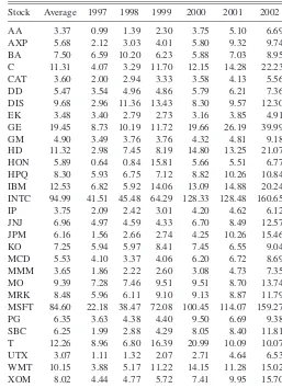
Table 10. Average number of trade quotations per minute of DJIA stocks
Stock Average 1997 1998 1999 2000 2001 2002
AA 3.37 0.99 1.39 2.30 3.75 5.10 6.69 AXP 5.68 2.12 3.03 4.01 5.80 9.32 9.74 BA 7.50 6.59 10.20 6.23 5.88 7.03 8.95 C 11.31 4.07 3.29 11.70 12.15 14.28 22.23 CAT 3.60 2.00 2.94 3.33 3.58 4.13 5.56 DD 5.47 3.54 4.96 4.86 5.79 6.21 7.36 DIS 9.68 2.96 11.36 13.43 8.30 9.57 12.30 EK 3.48 3.40 2.79 2.73 3.16 3.85 4.91 GE 19.45 8.73 10.19 11.72 19.66 26.19 39.99 GM 4.90 3.49 3.76 3.76 4.32 4.81 9.18 HD 11.32 2.98 7.45 8.19 14.80 13.25 21.07 HON 5.89 0.64 0.84 15.81 5.66 5.51 6.77 HPQ 8.30 5.93 6.75 7.12 8.82 10.26 10.84 IBM 12.53 6.82 5.92 14.06 13.09 14.88 20.24 INTC 94.99 41.51 45.48 64.29 128.33 128.48 160.65 IP 3.75 2.09 2.42 3.01 4.20 4.62 6.12 JNJ 6.96 4.97 4.59 4.33 6.70 8.49 12.57 JPM 6.16 1.56 2.66 2.74 4.25 10.26 15.46 KO 7.25 5.94 5.97 8.41 7.45 6.55 9.04 MCD 5.53 4.10 3.37 4.06 6.20 6.72 8.69 MMM 3.65 1.86 2.22 2.60 3.08 4.73 7.35 MO 9.39 7.28 7.46 9.51 9.51 8.70 13.74 MRK 8.48 5.96 6.11 9.10 9.13 8.87 11.79 MSFT 84.60 22.18 38.47 72.08 100.45 114.07 159.27 PG 6.35 3.63 4.38 4.40 9.50 6.69 9.38 SBC 6.25 1.99 2.88 4.29 8.05 8.40 11.81 T 12.26 8.96 6.80 16.39 20.99 10.09 10.07 UTX 3.07 1.11 1.32 2.07 2.71 4.64 6.53 WMT 10.15 3.88 5.17 11.22 14.15 11.28 15.02 XOM 8.02 4.44 4.77 5.72 7.41 9.95 15.70 Table 9. Names and symbols of the companies included in the DJIA
Company Ticker symbol
Alcoa Inc. AA
American Express Co. AXP
Boeing Co. BA
Citigroup Inc. C
Caterpillar, Inc. CAT
DuPont (E.I.) de Nemours DD
Walt Disney Co. DIS
Eastman Kodak Co. EK
General Electric Co. GE
General Motors GM
Home Depot Inc. HD
Honeywell Int’l. Inc. HON
Hewlett-Packard Co. HPQ
International Bus. Mach. IBM
Intel Corp. INTC
International Paper Co. IP
Johnson & Johnson JNJ
J.P. Morgan Chase & Co. JPM
Coca-Cola Co. KO
McDonald’s Corp. MCD
3M Company MMM
Altria Group, Inc. MO
Merck & Co.Inc. MRK
Microsoft Corp. MSFT
Procter & Gamble Co. PG
SBC Communications, Inc. SBC
AT&T Corp. T
United Technologies Corp. UTX
Wal-Mart Stores, Inc. WMT
Exxon Mobile Corp. XOM
January 1, 1997 until December 24, 2002, for a total of 1,505 trading days. Our sample contains the DJIA of individual firms as it was in 2000. The names and the symbols of the stocks included in the sample are reported in Table 9. Also, in our
empirical exampleT¼5 and therefore we have a total of 301 five-day periods.
Table 10 shows the average number of quotations per minute for all individual stocks. The table presents a spectrum of liq-uidity, ranging from as low as 3 quotations per minute for United Technologies Corp. (UTX) to as high as 94 for Intel Corp. The two most liquid stocks in the sample are Intel and Microsoft. Liquidity has increased substantially during the sample period and, as we approach 2002, the number of quo-tations per minute almost doubles for some stocks [e.g., 3M Company (MMM), Citigroup Inc. (C), Home Depot Corp. (HD), Microsoft (MSFT)].
From the original dataset, which includes prices recorded for every trade, we extracted 1 and 10 min interval data. Provided that there is sufficient liquidity in the market, the 5 min fre-quency is generally accepted as the highest frefre-quency at which the effect of microstructure biases are not too distorting (see Andersen et al. 2001; Andersen, Bollerslev, and Lange 1999; Ebens 1999); hence, the choice of the two mentioned fre-quencies to calculate the test statistics, to highlight the full extent of the microstructure noise effects.
The price series are determined using the last tick method, which was first proposed by Wasserfallen and Zimmermann (1985). Specifically, when no trade occurs at the required point in time, we use the last observed price. The New York Stock Exchange opens at 9:30 a.m. and closes at 4.00 p.m. Therefore, a full trading day consists of 390 (resp. 39) intraday returns calculated over an interval of one minute (resp. 10 minutes). Not all the days have the same number of price observations, because NYSE closes early on certain days, such as Christmas Eve; for all these intervals without price quotes we insert zero return values. This may have a bias toward not finding microstructure; however, the number of zeros is only an insignificant fraction of the total sample. When multiple prices are provided at the required time, we simply select the last.
Finally, for the most liquid stocks, namely INTC and MSFT, we have also considered ultra high frequencies (10 and 30 sec), as well as intermediate (2.5 and 5 min), and low (15 min) ones.
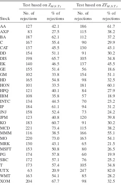
Figure 1. Plot of the test statistic defined in (8), with the 95% percentile of the standard normal (dotted line). Table 11. Results of the tests for assessing the effect of microstructure
noise (at the 5% level)
Stock
Test based onZM;N;T;t Test based onZTM;N;T;t
No. of rejections
% of rejections
No. of rejections
% of rejections
AA 127 42.1 186 61.7
AXP 83 27.5 115 38.2
BA 187 62.1 112 37.2
C 167 55.4 90 29.9
CAT 137 45.5 130 43.1
DD 154 51.1 91 30.2
DIS 198 65.7 105 34.8
EK 140 46.5 137 45.5
GE 155 51.4 56 18.6
GM 102 33.8 154 51.1
HD 165 54.8 98 32.5
HON 101 33.5 181 60.1
HPQ 121 40.1 84 27.9
IBM 108 35.8 57 18.9
INTC 134 44.5 70 23.2
IP 184 61.1 94 31.2
JNJ 158 52.4 73 24.2
JPM 123 40.8 120 39.8
KO 183 60.7 91 30.2
MCD 221 73.4 115 38.2
MMM 116 38.5 166 55.1
MO 220 73.0 163 54.1
MRK 130 43.1 65 21.5
MSFT 153 50.8 80 26.5
PG 174 57.8 60 19.9
SBC 172 57.1 76 25.2
T 173 57.4 105 34.8
UTX 63 20.9 247 82.0
WMT 163 54.1 85 28.2
XOM 204 67.7 98 32.5
4.2 Assessing the Effects of Microstructure Noise
Because ZM;N;T;t andZTM;N;T;t have a normal limiting
dis-tribution over a finite time spanT;we have sequentially run the statistics over consecutive 5-day periods. WithMandNfinite, it may well occur that in certain periods we reject the null, whereas in others we fail to reject. In principle, we could compare thepvalues over the various subperiods and construct Bonferroni type bounds. However, given the high degree of correlation acrosspvalues, we cannot rely too much on these types of bounds. Furthermore, they are very conservative. Thus, in Table 11, columns 2–5, we simply report the per-centage of 5-day periods in which we did reject the null of no
noise contamination, based on the statistic defined in (8) and (11), respectively. Overall, we find strong evidence of micro-structure effects for most of the stocks.
Overall, we do not find evidence of a clear relationship between liquidity and microstructure effects. For example, in a liquid stock like Intel, the null was rejected 44.5% of the times. For a relatively illiquid stock such as XOM, microstructure was significant 67.7% of the periods. In Figure 1, we report the plot of the test statistic over the different 5-day intervals considered, with the dotted lines representing the 5% upper and lower tail critical values of a standard normal. We notice that there are a few instances in which the statistic has a large negative value.
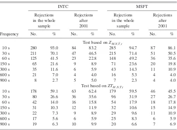
Table 12. Results of the tests for assessing the effect of microstructure noise (at the 5% level) comparing different frequencies withNcorresponding to 20 min
Frequency
INTC MSFT
Rejections in the whole
sample
Rejections after 2001
Rejections in the whole
sample
Rejections after 2001
No. % No. % No. % No. %
Test based onZM;N;T;t
10 s 280 93.0 84 83.2 285 94.7 87 86.1
30 s 211 70.1 47 46.5 215 71.4 51 50.5
60 s 125 41.5 23 22.8 148 49.2 36 35.6
150 s 65 21.6 9 8.9 71 23.6 20 19.8
300 s 35 11.6 6 5.9 43 14.3 11 10.9
600 s 21 7.0 4 4.0 16 5.3 4 4.0
900 s 8 2.7 5 5.0 7 2.3 4 4.0
Test based onZTM;N;T;t
10 s 178 59.1 63 62.4 179 59.5 46 45.5
30 s 80 26.6 36 35.6 96 31.9 27 26.7
60 s 42 14.0 16 15.8 54 17.9 18 17.8
150 s 31 10.3 12 11.9 32 10.6 15 14.9
300 s 22 7.3 9 8.9 29 9.6 11 10.9
600 s 17 5.6 6 5.9 25 8.3 6 5.9
900 s 19 6.3 10 9.9 20 6.6 7 6.9
Figure 2. Plot of the test statistic defined in (11), with the 95% percentile of the standard normal (dotted line).
This happens mainly when the microstructure noise is neg-atively correlated with the efficient price, thus introducing a negative bias in volatility measurement. In January 2001, the tick size was reduced from 1/16 to 1/100 of a dollar, and this has affected the magnitude of the variance of microstructure noise (see Bandi and Russell 2006, 2007; Corradi, Distaso, and Swanson 2006). We have divided our sample into two sub-samples (pre- and post-tick decimalization) to check whether the reduction in the tick size had an impact on the rejection rates (results are not reported in Tables for space reasons). There were 77.6% rejections, which occurred before tick decimalization, whereas the sample size before January 2001 accounted for 66.6% of the total sample. Hence, we can conclude that tick decimalization has attenuated the effect of microstructure noise. Table 11, columns 4 and 5, report the results for the test based on the statistic defined in (11). We notice that the rejection rates are generally smaller than those obtained using the previous test. As the latter statistic is robust to the presence of large and rare jumps, the obtained results seem to provide evidence in favor of the fact that some of the 5-day periods are affected by jumps for most stocks. These results are consistent
with the empirical findings of Andersen et al. (2005) and Huang and Tauchen (2005). However, for AA, AYP, GM, HON, MMM, UTY we notice that rejection rates coming from the test based onZTM;N;T;t are substantially higher than those of
the test based onZM;N;T;t :This can be the result of some size
distortion induced by jumps. In fact, in the numerator, the effect of the pure jump component, which is the same for both RVt;T;N andRVt;T;M ; cancels out. However, the effect of the
pure jump component in the denominator, the estimated quarticity, is of orderpffiffiffiffiffiffiffiNT:
The plot of the test statistic (for some selected stocks), for each 5-day interval, is inserted in Figure 2.
Table 12 reports the results of the same tests, obtained comparing different frequencies with N corresponding to 20 min. Results are reported only for MSFT and INTC, the most liquid stocks, given the high frequencies considered. The table reveals some interesting facts. The test based onZM;N;T;t starts
rejecting the null hypothesis when the sampling frequency approaches 2.5 min. For higher frequencies, rejection rates become quite high. Also, one can appreciate the effect of the tick decimalization clearly here. When we run the test at low Table 13. Results of the unconditional test based onVM;N;L;T;t(at the 5% level)
Stock
Frequencies
60 s versus 150 s
150 s versus 300 s
60 s versus 600 s
150 s versus 600 s
300 s versus 600 s
Rejections Rejections Rejections Rejections Rejections
No. % No. % No. % No. % No. %
AA 9 3.0 2 0.7 25 8.3 14 4.6 7 2.3
AXP 9 3.0 2 0.7 25 8.3 18 5.9 7 2.3
BA 12 4.0 2 0.7 23 7.6 16 5.3 8 2.6
C 6 2.0 3 1.0 23 7.6 18 5.9 8 2.6
CAT 5 1.7 7 2.3 20 6.6 16 5.3 7 2.3
DD 7 2.3 2 0.7 30 9.9 24 7.9 12 3.9
DIS 11 3.7 0 0.0 20 6.6 17 5.6 7 2.3
EK 8 2.7 1 0.3 24 7.9 14 4.6 6 1.9
GE 9 3.0 0 0.0 18 5.9 13 4.3 6 1.9
GM 10 3.3 1 0.3 22 7.3 17 5.6 11 3.6
HD 4 1.3 0 0.0 23 7.6 15 4.9 5 1.6
HON 6 2.0 0 0.0 19 6.3 12 3.9 3 0.9
HPQ 6 2.0 0 0.0 26 8.6 18 5.9 5 1.6
IBM 10 3.3 0 0.0 21 6.9 10 3.3 4 1.3
INTC 11 3.7 1 0.3 34 11.2 25 8.3 14 4.6
IP 10 3.3 2 0.7 24 7.9 15 4.9 9 2.9
JNJ 13 4.3 0 0.0 28 9.3 20 6.6 13 4.3
JPM 17 5.6 0 0.0 32 10.6 22 7.3 8 2.6
KO 11 3.7 1 0.3 21 6.9 18 5.9 11 3.6
MCD 14 4.7 1 0.3 32 10.6 26 8.6 12 3.9
MMM 10 3.3 2 0.7 23 7.6 19 6.3 11 3.6
MO 22 7.3 3 1.0 30 9.9 19 6.3 10 3.3
MRK 8 2.7 2 0.7 21 6.9 18 5.9 8 2.6
MSFT 14 4.7 3 1.0 31 10.2 21 6.9 12 3.9
PG 10 3.3 1 0.3 34 11.2 20 6.6 12 3.9
SBC 13 4.3 1 0.3 34 11.2 30 9.9 14 4.6
TT 14 4.7 3 1.0 32 10.6 25 8.3 12 3.9
UTX 7 2.3 0 0.0 22 7.3 14 4.6 8 2.6
WMT 13 4.3 2 0.7 25 8.3 15 4.9 5 1.6
XOM 16 5.3 1 0.3 39 12.9 34 11.2 15 4.9
frequencies, there is not much difference between rejection rates over the entire sample (columns 3 and 7) and those over the pre-2001 sample (columns 5 and 9). Conversely, at higher frequencies we see a more marked difference, which is atte-nuated again at the ultra high frequency of 10 sec. Results are very similar for INTC and MSFT.
Moving to the test based on ZTM;N;T;t ; we notice some
important differences. For frequencies of 2.5 min and higher, rejection rates are substantially smaller than those of the other test. Furthermore, apart from the 10 sec frequency, there seems to be no appreciatable effect of tick decimalization.
When running the tests with the different frequencies, we have also recorded the highest frequency at which we do not reject the null hypothesis, for each of the 301 five-day periods (for space reasons, results are not reported in Tables). Here, we only com-ment on the results for Intel, because those for Microsoft are qualitatively similar and are omitted for space reasons. Starting from the test based onZM;N;T;t ;we see that, for the entire sample,
the average frequency at which we do not reject is 171 sec, and the mode is reached at the frequency of 60 sec (26.9%). The average frequency, as expected, is lower (205 sec) for the period before tick decimalization and rises to 102 sec afterward.
Mirroring the results of Table 12, the average frequency for the test based onZTM;N;T;t is 98 sec (for the entire sample),
and the mode is at 30 sec (41.5%). Again, the effect of tick decimalization appears to be less marked in this case, with the average frequencies being equal, respectively, to 102 (pre-January 2001 sample) and 89 sec (post-(pre-January 2001 sample).
4.3 A Specification Test for the Variability of the Microstructure Noise
In this subsection, we test H00 versus H0A;defined, respec-tively, in (16) and (17), using the statistic suggested in (18). We perform three sequences of test, the first one conditional on rejecting the null of no microstructure using the test statistic in (8), the second conditional on the same outcome using the statistic in (11), and then an unconditional one. Here, we only comment on the unconditional test (Table 13), because the findings for the conditional tests are very similar.
Rejections of the null hypothesis, up to the one minute sampling interval, are not very frequent. One could think that the results of columns 6 and 7 in the Table are a result of some lack of power of the tests (the rate of divergence of the test is pffiffiffiffiffiffiffiNT; i.e., it is driven by the lower frequency). But columns 2 and 3 confirm and robustify the findings. The Table suggests that the model of iid microstructure noise with constant variance frequently adopted by the literature is a good candidate for describing the features of the microstructure effects. This is quite intuitive because, for example, the mag-nitude of the bid-ask spread or the distortion induced by price discreteness do not depend on the sampling frequency.
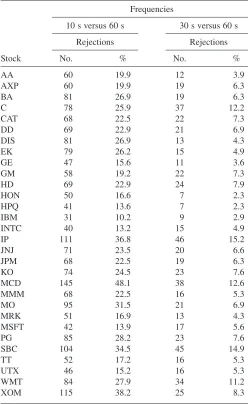
The picture changes when we move to ultra high frequen-cies. Table 14 reports the results of the test comparing the 1 min frequency to 30 and 10 sec. When comparing 1 min to 30 sec, only five stocks exceed 10% of rejections, whereas for the case of 1 min versus 10 sec all the stocks are above the 10% of rejections, with 5 above 30% and 13 between 20% and 30%.
Our results are consistent with the previous literature, which finds that the i.i.d. assumption is justifiable for a sampling frequency up to one-minute, but then inadequate at ultra-high frequencies.
5. CONCLUDING REMARKS
While the increasing availability of high frequency data provides a valuable opportunity for the calculation of model-free estimators of asset return volatility, the presence of market microstructure noise could seriously undermine the validity of such estimators.
Based on a comparison between two realized volatilities computed over different frequencies, we develop a test for the null hypothesis of no microstructure noise and establish its asymptotic properties. Then, if the null hypothesis is rejected, we propose a specification test for the hypothesis that the variability of the microstructure noise is independent of the frequency over which data are sampled.
Our theory is applied to the DJIA stocks, for the period 1997–2002. The evidence suggests that the effect of micro-structure noise on volatility estimators starts to be statistically significant at frequencies between 2 and 3 min.
Table 14. Results of the unconditional test based onVM;N;L;T;t
(at the 5% level)
Stock
Frequencies
10 s versus 60 s 30 s versus 60 s
Rejections Rejections
No. % No. %
AA 60 19.9 12 3.9
AXP 60 19.9 19 6.3
BA 81 26.9 19 6.3
C 78 25.9 37 12.2
CAT 68 22.5 22 7.3
DD 69 22.9 21 6.9
DIS 81 26.9 13 4.3
EK 79 26.2 15 4.9
GE 47 15.6 11 3.6
GM 58 19.2 22 7.3
HD 69 22.9 24 7.9
HON 50 16.6 7 2.3
HPQ 41 13.6 7 2.3
IBM 31 10.2 9 2.9
INTC 40 13.2 15 4.9
IP 111 36.8 46 15.2
JNJ 71 23.5 20 6.6
JPM 68 22.5 19 6.3
KO 74 24.5 23 7.6
MCD 145 48.1 38 12.6
MMM 68 22.5 16 5.3
MO 95 31.5 21 6.9
MRK 51 16.9 13 4.3
MSFT 42 13.9 17 5.6
PG 85 28.2 23 7.6
SBC 104 34.5 45 14.9
TT 52 17.2 16 5.3
UTX 46 15.2 16 5.3
WMT 84 27.9 34 11.2
XOM 115 38.2 25 8.3
As for the properties of the noise, the widely used constant variance iid specification seems to be plausible for frequencies up to 1 min/30 sec, but then it is not empirically supported at ultra high frequencies.
APPENDIX
A.1 Proof of Proposition 1
(1) The statistic defined in (8) can be expanded into
ZM;N;T;t ¼
The central limit theorems in Jacod (1994) and Jacod and Protter (1998) established that, asM!‘,
ffiffiffiffiffiffiffiffi
‘, N/M ! 0. As a consequence, the limiting distribution of
ZM;N;T;t under H0will be determined by the second component of (A.1). By a similar argument as before, because, asN!‘,
the statement follows immediately.
(2) Under the alternative hypothesis, it is possible to expand the components in the numerator of (A.1), re-spectively, as
Therefore, the statistic will diverge to plus infinity and the test will be consistent if, asN,M!‘,
which holds under Assumption A4.
In fact, the left of (A.2) is of probability order
MbM1NbN1
which approaches infinity, given Assumption A4.
A.2 Proof of Proposition 2
(1) From Barndorff-Nielsen et al. (2006, Theorem 2.3), if there are no jumps in the return process, asM!‘,
whereais defined as in (12). Also,
QVt;T;M !
p Z tþT t
s4sds: ðA:4Þ In the presence of jumps in the return process, providedJtis a
finite activity counting process, it follows by Proposition 1 in Barndorff-Nielsen, Shephard, and Winkel (2006) that the central limit result stated in (A.3) still holds. The statement then comes by the same argument used in the proof of Prop-osition 1(1).
(2) By the same argument used in the proof of
Proposi-tion 1 (2). j
A.3 Proof of Proposition 3
(1) Under the null,
ffiffiffiffiffiffiffiffi
as over a finite time span the drift term is bounded with probability one. Also, by a similar argument as in the proof of Theorem 1 in Barndorff-Nielsen et al. (2006),
ffiffiffiffiffiffiffiffi
and
Finally, given (A.4), the statement follows.
(2) Recalling A4, the numerator diverges to minus infinity at rateMbMand the numerator diverges at rate
ffiffiffiffiffiffiffiffiffiffi
MbM
p
:
A.4 Proof of Proposition 4
(1) Under the null hypothesis, the test statistic is asymp-totically equivalent to
By Theorem A1 in Zhang et al. (2005),
ffiffiffiffiffiffiffiffi because it converges in distribution. Thus,
VM;N;T;t ¼ pffiffiffiffiffiffiffiNT
Now, by Theorem A1 in Zhang et al. (2005),
ffiffiffiffiffiffiffi
is a consistent estimator for E e4
t :Thus, it follows that
VM;N;T;t¼ pffiffiffiffiffiffiffiNT
(2) Under the alternative hypothesis, the statistic can be rearranged as
Note that the first term on the right of (A.7) is asymptotically normal. As the second term on the right of (A.7) is of proba-bility orderpffiffiffiffiN nt;M
nt;N1
;it diverges to –‘.
Finally, robustness to jumps is easily established. The numerator of (A.6) can be rewritten as
pffiffiffiffiffiffiffiNT the denominator. Thus, the contribution of the jump component is asymptotically negligible, if the jump process is of finite activity.
ACKNOWLEDGMENTS
The authors thank the Editor, Torben Andersen, an asso-ciate editor, and two anonymous referees for helpful com-ments. We also thank Andrew Chesher, Peter Hansen, Bruce Lehmann, Asger Lunde, Theo Nijman, Bas Werker, the seminar participants at ICMA Centre in Reading, and the participants at the 2004 ‘‘Econometrics of Microstructure of Financial Markets’’ Workshop at CentER-Tilburg University, the 2004 North American Summer meeting and Australasian meeting of the Econometric Society, the 2004 UK Econo-metric Study Group, and the Quantitative Methods in Fin-ance 2004 Conference in Sydney for helpful comments and
suggestions. The authors gratefully acknowledge financial support from the ESRC, grant codes R000230006 and RES-062-23-0311.
[Received September 2007. Revised November 2007.]
REFERENCES
Aı¨t-Sahalia, Y., and Mancini, L. (2008). ‘‘Out-of-Sample Forecasts of Quad-ratic Variation,’’Journal of Econometrics, 147, 17–33.
Aı¨t-Sahalia, Y., Mykland, P. A., and Zhang, L. (2005), ‘‘How Often to Sample a Continuous Time Process in the Presence of Market Microstructure Noise,’’
Review of Financial Studies,18, 351–416.
——— (2006). ‘‘Ultra High Frequency Volatility Estimation with Dependent Microstructure Noise,’’ working paper, Princeton University.
Andersen, T. G., Bollerslev, T., Diebold, F. X., and Ebens H. (2001), ‘‘The Distribution of Realized Stock Returns Volatility,’’ Journal of Financial Economics, 61, 43–76.
Andersen, T. G., Bollerslev, T., Diebold, F. X., and Labys P. (2000), ‘‘Great Realizations,’’Risk, 105–108.
——— (2001), ‘‘The Distribution of Realized Exchange Rate Volatility,’’
Journal of the American Statistical Association, 96, 42–55.
——— (2003), ‘‘Modelling and Forecasting Realized Volatility,’’ Econo-metrica, 71, 579–625.
Andersen, T. G., Bollerslev, T., and Lange, S. (1999), ‘‘Forecasting Financial Market Volatility. Sample Frequency vs Forecast Horizon,’’ Journal of Empirical Finance,6, 457–477.
Andersen, T. G., Bollerslev, T., and Meddahi, N. (2004), ‘‘Analytical Evaluation of Volatility Forecasts,’’International Economic Review,45, 1079–1110. ——— (2006). ‘‘Realized Volatility Forecasting and Market Microstructure
Noise,’’ working paper, Northwestern University, Kellogg Business School. Bai, X., Russell, J. R., and Tiao, G. (2000). ‘‘Effects of Nonnormality and Dependence on the Precision of Variance Estimates Using High Frequency Data,’’ working paper, University of Chicago, Graduate School of Business. Bandi, F. M., and Russell, J. R. (2006), ‘‘Separating Microstructure Noise from
Volatility,’’Journal of Financial Economics,79, 655–692.
——— (2007). ‘‘Market Microstructure Noise, Integrated Variance Estimators, and the Accuracy of Asymptotic Approximations,’’ working paper, Uni-versity of Chicago, Graduate School of Business.
——— (2008), ‘‘Microstructure Noise, Realized Volatility, and Optimal Sampling,’’The Review of Economic Studies,75, 339–369.
Barndorff-Nielsen, O. E., Graversen, S. E., Jacod, J., Podolskij M., and Shephard N. (2006). ‘‘A Central Limit Theorem for Realised Power and Bipower Variations of Continuous Semimartingales,’’ inFrom Stochastic Analysis to Mathematical Finance, Festschrift for Albert Shiryaev,(eds) Y. Kabanov, R. Lipster, and J. Stoyanov, New York: Springer, pp. 33–68. Barndorff-Nielsen, O. E., Graversen, S. E., Jacod, J., and Shephard N. (2006).
‘‘Limit Theorems for Bipower Variation in Financial Econometrics,’’
Econometric Theory,22, 677–719.
Barndorff-Nielsen, O. E., Hansen, P. R., Lunde, A., and Shephard N. (2008). ‘‘Designing Realised Kernels to Measure the Ex-Post Variation of Equity Prices in the Presence of Noise,’’Econometrica, 76, 1481–1536.
——— (2009). ‘‘Subsampling Realised Kernels,’’Journal of Econometrics, (forthcoming).
Barndorff-Nielsen, O. E., and Shephard, N. (2002), ‘‘Econometric Analysis of Realized Volatility and Its Use in Estimating Stochastic Volatility Models,’’
Journal of the Royal Statistical Society: Series B,64, 253–280.
——— (2003), ‘‘Realized Power Variation and Stochastic Volatility,’’ Ber-noulli,9, 243–265.
——— (2004), ‘‘Power and Bipower Variation with Stochastic Volatility and Jumps (with discussion),’’Journal of Financial Econometrics,2, 1–48. ——— (2006), ‘‘Econometrics of Testing for Jumps in Financial Economics
Using Bipower Variation,’’Journal of Financial Econometrics,4, 1–30. Barndorff-Nielsen, O. E., Shephard, N., and Winkel, M. (2006), ‘‘Limit
The-orems for Multipower Variation in the Presence of Jumps,’’ Stochastic Processes and their Applications,116, 796–806.
Black, F. (1986), ‘‘Noise,’’The Journal of Finance,XLI, 529–543.
Bollen, B., and Inder, B. (2002), ‘‘Estimating Daily Volatility in Financial Markets Utilizing Intraday Data,’’Journal of Empirical Finance,9, 551– 562.
Corradi, V., Distaso, W., and Swanson, N. R. (2006). ‘‘Predictive Inference for Integrated Volatility,’’ working paper, University of Warwick.
Ebens, H. (1999). ‘‘Realized Stock Volatility,’’ working paper, John Hopkins University.
Ghysels, E., and Sinko, A. (2006), ‘‘Comment on Hansen and Lunde,’’Journal of Business & Economic Statistics,24, 192–194.
Gloter, A., and Jacod, J. (2001a), ‘‘Diffusions with Measurement Errors. I-Local Asymptotic Normality,’’ESAIM: Probability and Statistics,5, 225–242. ——— (2001b), ‘‘Diffusions with Measurement Errors. II-Optimal
Estima-tors,’’ESAIM: Probability and Statistics,5, 243–260.
Hansen, P. R., Large, J., and Lunde, A. (2006), ‘‘Moving Average-Based Estimators of Integrated Variance,’’Econometric Reviews,27, 79–111. Hansen, P. R., and Lunde, A. (2006), ‘‘Realized Variance and Market
Micro-structure noise (with comments and rejoinder),’’ Journal of Business & Economic Statistics,24, 127–218.
Hasbrouck, J. (1993), ‘‘Assessing the Quality of a Security Market. A New Approach to Transaction Cost Measurement,’’Review of Financial Studies,
6, 191–212.
Hasbrouck, J., and Seppi, D. (2001), ‘‘Common Factors in Prices, Order Flows, and Liquidity,’’Journal of Financial Economics,59, 383–411.
Huang, X., and Tauchen, G. (2005), ‘‘The Relative Contribution of Jumps to Total Price Variation,’’ Journal of Financial Econometrics,3, 456– 499.
Jacod, J. (1994). ‘‘Limit of Random Measures Associated with the Increments of a Brownian Semi-Martingale. Preprint number 120, Paris: Laboratoire de Probabilitie´s, Universite´ Pierre et Marie Curie.
Jacod, J., and Protter, P. (1998), ‘‘Asymptotic Error Distributions for the Euler Method for Stochastic Differential Equations,’’Annals of Probability,26, 267–307.
Karatzsas, I., and Shreve, S. E. (1991).Brownian Motion and Stochastic Cal-culus.New York: Springer Verlag.
Meddahi, N. (2002), ‘‘A Theoretical Comparison between Integrated and Realized Volatility,’’Journal of Applied Econometrics,17, 475–508. O’Hara, M. (2003), ‘‘Presidential Address: Liquidity and Price Discovery,’’The
Journal of Finance,LVIII, 1335–1354.
Oomen, R. C. (2005), ‘‘Properties of Bias-Corrected Realized Variance Under Alternative Sampling Schemes,’’Journal of Financial Econometrics,3, 555– 577.
——— (2006), ‘‘Properties of Realized Variance Under Alternative Sampling Schemes,’’Journal of Business & Economic Statistics,24, 219–237. Protter, P. (1990).Stochastic Integration and Differential Equations.New York:
Springer Verlag.
Wasserfallen, W., and Zimmermann, H. (1985), ‘‘The Behavior of Intraday Exchange Rates,’’Journal of Banking & Finance,9, 55–72.
Zhang, L. (2006), ‘‘Efficient Estimation of Stochastic Volatility Using Noisy Observations: A Multi-Scale Approach,’’Bernoulli,12, 1019–1043. Zhang, L., Mykland, P. A., and Aı¨t-Sahalia, Y. (2005), ‘‘A Tale of
Two Time Scales: Determining Integrated Volatility with Noisy High Fre-quency Data,’’Journal of the American Statistical Association,100, 1394– 1411.