Full Terms & Conditions of access and use can be found at
http://www.tandfonline.com/action/journalInformation?journalCode=ubes20
Download by: [Universitas Maritim Raja Ali Haji] Date: 13 January 2016, At: 00:20
Journal of Business & Economic Statistics
ISSN: 0735-0015 (Print) 1537-2707 (Online) Journal homepage: http://www.tandfonline.com/loi/ubes20
How Do Behavioral Assumptions Affect
Structural Inference? Evidence From a Laboratory
Experiment
Daniel Houser & Joachim Winter
To cite this article: Daniel Houser & Joachim Winter (2004) How Do Behavioral Assumptions
Affect Structural Inference? Evidence From a Laboratory Experiment, Journal of Business & Economic Statistics, 22:1, 64-79, DOI: 10.1198/073500103288619386
To link to this article: http://dx.doi.org/10.1198/073500103288619386
View supplementary material
Published online: 01 Jan 2012.
Submit your article to this journal
Article views: 54
How Do Behavioral Assumptions
Affect Structural Inference?
Evidence From a Laboratory Experiment
Daniel H
OUSERInterdisciplinary Center for Economic Science & Department of Economics, George Mason University, Fairfax, VA 22030 (dhouser@gmu.edu)
Joachim W
INTERMannheim Research Institute for the Economics of Aging, University of Mannheim, D-68131 Mannheim, Germany (winter@uni-mannheim.de)
We use laboratory experiments to investigate the effect that assuming rational expectations has on struc-tural inference in a dynamic discrete decision problem. Our design induces preferences up to the subjective rate of time preference, leaving unrestricted both this parameter and subjects’ decision rules. We estimate subjects’ discount rates under the assumption that all subjects use the rational expectations decision rule, and under weaker behavioral assumptions that allow decision rule heterogeneity. We nd that certain sophisticated heuristics t subjects’ decisions statistically signicantly better than rational expectations. However, the rational expectations assumption does not distort inferences about the cross-sectional dis-count rate distribution.
KEY WORDS: Discounting; Heterogeneity; Heuristics; Rational expectations; Search; Statistical clas-sication algorithm.
1. INTRODUCTION
The latter half of the twentieth century saw the emergence of a large literature documenting apparently irrational behav-ior by subjects in economics and psychology experiments. This has led theorists, particularly over the last 10 years, to be-gin to assess the equilibrium implications of certain types of rule-of-thumb behavior (see, e.g., Ellison and Fudenberg 1993; Krusell and Smith 1995; Lettau and Uhlig 1999; Anderlini and Canning 2001). Interestingly, however, relatively little effort has been made by empirical economists to understand whether, as a practical matter, assuming rational expectations leads to misspecied models that substantially distort inferences about structural parameters. A reason for this is that both the analy-sis of eld data and simulation procedures are limited in the extent to which they can address this issue. This article uses a laboratory experiment to investigate the sensitivity of infer-ences about one structural parameter—the subjective rate of time preference—to the rational expectations assumption.
The experimental laboratory has proved a useful tool for in-vestigating statistical questions not easily answered through the analysis of eld data or Monte Carlo simulations. For example, Cox and Oaxaca (1999) recently used lab experiments to as-sess whether supply-and-demand parameters can be recovered from data generated by various common market institutions. They pointed out that standard procedures to recover these pa-rameters require assumptions about the data-generating process (DGP), and, to the extent that these assumptions generate spec-ication errors, inferences can be erroneous. Whereas Monte Carlo simulations can be used to study the effects of any par-ticular misspecication, the DGPs considered in such exercises might not correspond to any naturally occurring DGP. Cox and Oaxaca (1999) pointed out that one advantage of the experi-mental laboratory is that it can be used to study the effects of the specic misspecication that arises when the true DGP stems
from human behavior. Our study, which examines the effects of different expectations specications, takes advantage of this feature of laboratory experiments.
Rational expectations is the standard assumption in virtually all applied structural econometric work, and this has generated some criticism. As Blundell (1994, p. 4) pointed out, “struc-tural models are often accused (in many cases quite rightly) of imposing untenable and unbelievable restrictions on behavior.” Nevertheless, there seems to be very little evidence suggesting that the rational expectations assumption has had detrimental effects in any positive sense. Research using eld data to es-timate life-cycle labor supply models with expectations-robust procedures (see, e.g., Hotz and Miller 1988; Houser 2003) typ-ically obtains results that line up well with results based on ra-tional expectations specications.
Unfortunately, there is a fundamental limitation to the amount that one can learn about the effect of expectation speci-cation errors from the analysis of eld data. In particular, Rust (1994) showed that under very general conditions, individuals’ preferences and their expectations processes are jointly non-parametrically unidentied. Because persons’ true period return functions are not generally known, and because the identica-tion problem implies that multiple period return funcidentica-tion and expectation specication combinations will t the data equally well in-sample, examining the consequences of expectation misspecication with eld data presents a substantial challenge. In contrast, the experimental laboratory provides an environ-ment in which period return functions can be controlled,and the identication problem consequentlycircumvented.The result is
© 2004 American Statistical Association Journal of Business & Economic Statistics January 2004, Vol. 22, No. 1 DOI 10.1198/073500103288619386 64
that inferences about the effect of expectation misspecication on structural inference become possible.
This article analyzes data from a price search experiment that induces preferences (but not the way in which people form ex-pectations) up to a single structural parameter: the rate of sub-jective time preference (or the “subsub-jective discount rate”). Our experimental design, which builds on work of Rapoport and Tversky (1970) and Seale and Rapoport (1997), provides in-formation on discount rates because it incorporates the possi-bility that a subject’s experimental earnings might be paid to them 2 weeks after they complete their laboratory session. In-ferences about time preference have been drawn in many other laboratory experimental studies; Frederick, Loewenstein, and O’Donoghue (2002) have provided a comprehensive review of this literature. A recent study by Warner and Pleeter (2001) took advantage of a natural experiment, providing data on real choices with large stakes, to estimate time discount rates. Fi-nally, some econometric studies have estimated discount rates from eld data using indirect inference methods (e.g., Lang and Ruud 1986; Samwick 1998; Gourinchas and Parker 2001; Cagetti 2003). In contrast to these studies, our focus is not so much on estimating the discount rate per se, but rather on un-derstanding the interaction of assumptions about individuals’ behavior and such estimates.
We compare three approaches to inference about subjects’ discount rates. One assumption common to each approach is that subjects are risk neutral. This assumption is standard in the price search literature, and using it here allows our results to be more easily compared to that literature. Moreover, although preferences regarding risk and intertemporal substitution can be separately conceptualized in abstract models, say, using the framework of Kreps and Porteus (1978), they are typically dif-cult to distinguish in practice. Still the assumption of risk neu-trality might fail. Because risk-averse subjects should stop the search sooner on average, and because it turns out that more im-patient subjects should also stop the search sooner on average, the failure of risk neutrality would tend to bias our discount rate estimates downward.
Our rst results are derived from a simple revealed prefer-ence analysis based on subjects’ accepted payoffs only. This procedure enables us to establish discount rate bounds under the weak assumption that subjects prefer higher payoffs to lower payoffs (and that they are risk neutral). Although this procedure is robust, it ignores all continuation decisions that, in general, also contain information about discount rates. In particular, a subject’s stopping rule within the sequential search task will vary with his on her rate of time preference, both under rational expectations and under many alternative decision rules (which we call “heuristics” in the sequel). Incorporating stronger be-havioral assumptions, therefore, typically allows more precise inference about rates of time preference, albeit at the possible cost of bias due to model misspecication.
Our second set of results is derived using a very strong be-havioral assumption, namely that subjects have rational expec-tations. Although evidence shows that people do not behave according to rational expectations in many dynamic decision tasks (see, e.g., Carbone and Hey 1999), other studies (e.g., Hey 1982) have found that behavior in price-search tasks is often
quite close to optimal. This is an important advantage of our de-sign, because in our view, people likely behave nearly optimally in many actual intertemporal (life-cycle) decision problems.
The nal set of results is based on a more robust approach that is relatively common in experimental game theory (e.g., Weber and Tietz 1975; Selten 1991). We specify a set of candi-date decision rules from which the decision rule that best ts ob-served behavior is selected for each subject. Similar ideas have been explored by Hey (1981, 1982, 1987) and Moon and Mar-tin (1990) in the experimental analysis of price-search prob-lems, and by Müller (2001) in an experiment on behavior in life-cycle choice situations. In our case, the set of candidate de-cision rules includes the optimal, rational expectations dede-cision rule as well as various more- or less-sophisticated heuristics. The main difference between earlier studies and our approach is that for each subject, we jointly determine both the decision rule and a structural parameter (the subjective discount rate). Moreover, in contrast to the literature cited earlier, we use a formal statistical estimation approach rather than informal clas-sication procedures. Our estimation procedure, related to that of El-Gamal and Grether (1995), relaxes both the assumption of rational expectations and the assumption that all subjects use the same decision rule. At the same time, as we explain in Sec-tion 5, our procedure avoids the problem of overtting.
Relative to the revealed preference analysis, we nd that im-posing behavioral restrictions substantially sharpens inferences about discount rates. We also show that the data are described less well by rational expectations behavior than by simpler heuristics. The reason is that subjects tend to stop searching sooner on average than is consistent with rational expectations behavior and low time discounting (i.e., high willingness to ac-cept delayed payoffs). At the same time, rational expectations behavior under high time discounting is inconsistent with the frequency of delayed payoffs that are accepted. It turns out that some of the heuristics that we consider accommodate both re-laxed stopping criteria and little time discounting,and it is these heuristics that best explain our data. Nevertheless, we do not nd statistically signicant differences between the estimates of the cross-sectional distribution of discount rates that emerge under rational expectations and weaker behavioral assumptions (heuristics). The mean and median of the estimates are .65 and .68 under the rational expectations analysis and both .70 under weaker behavioral assumptions.
Although population-level inference seems robust to behav-ioral specications, inferences about any given individual’s discount rate can vary substantially across behavioral speci-cations. We cannot know any subject’s true rate of time pref-erence, but nevertheless we can investigate the relationship between subjects’ estimated discount rates and an external mea-sure of the extent to which they are forward-looking. The ex-ternal measure that we use is based on a personality survey, described in detail below, that we administered as part of the price-search experiment. We nd that neither revealed prefer-ence nor rational expectations estimates are statistically sig-nicantly correlated with this external measure, whereas our heuristic-based discount rate estimates and the external mea-sure are statistically signicantly positively correlated.
The remainder of the article is structured as follows. In Sec-tion 2 we introduce our experimental design. We then present
evidence of discounting and derive bounds on subjective dis-count rates in Section 3. In Sections 4 and 5 we discuss struc-tural inference about discount rates under rational expectations and under weaker behavioral assumptions, respectively. In Sec-tion 6 we discuss differences between the estimates at both the aggregate and individual levels. We provide some concluding remarks in Section 7.
2. EXPERIMENTAL DESIGN
In our experiment, subjects make decisions in a standard price-search problem (Rapoport and Tversky 1970; Seale and Rapoport 1997) modied to incorporate delayed payments. Each subject’s goal is to purchase a “widget” that they value at 100 tokens. The widget is sold at many different locations, and visiting a new location costs one token. Each location posts both a price and availability (today or in 14 days) for the widget; this location-specic information is revealed when the subject visits that location. Subjects are informed that the price at each location is drawn independentlyfrom a normal distribution with a mean of 100 and standard deviation of 10. Subjects are also informed that the availability at each location is drawn inde-pendently (both across locations and with respect to the price draw); availabilityis immediate with probability.5 or in 14 days with probability .5. Subjects may stop their search at any time and purchase the widget from any of the locations that they vis-ited. (Hence this it is a search problem “with recall”.) An exact transcript of the instructions for this experiment, along with all data used in this article, are provided on theJBESwebsite.
This design allows inference about time preference within an environment where past research has shown behavior to be nearly rational. Experiments conducted by Hey (1982, 1987) have suggested that search behavior is closer to optimal when there is no recall and when subjects have full information about the price distribution. Our design combines the possibility of recall and the availability of information about the price distri-bution. We do this because (1) the possibility of recall together with the time-differentiated availability of the product (and pos-sibility of a delayed payment of the search surplus) allows us to observe within-game trade-offs between different points in time, and (2) giving subjects full knowledge about the price distribution, along with the opportunity to become experienced with the task, avoids problems arising from learning about the parameters of the price distribution that might distort inference about time preference.
The perception that delayed payment involves risks or trans-action costs can bias inference about a subject’s rate of time preference. We designed the experiment with these concerns in mind. Specically, subjects were told that at the end of the ex-periment, their earnings would be put into an envelope. If they chose an immediate payment, then the envelope would be given to them immediately. If they chose a delayed payment, their en-velope would be stored in a safe until it was delivered or picked up in 14 days. The instructions read: “We absolutely guarantee that 14 days from today you will be able to obtain your enve-lope with your earnings. Moreover, we will pay any costs (such as mailing costs) required to get your earnings to you after 14 days.”
The experiment was conducted at the University of Arizona’s Economic Science Laboratory in the Spring and Summer of 2000. Subjects were recruited from the general student popu-lation. All experiments were run entirely on computers using Visual Basic software written by the authors. (This software is available from either author on request.)
Upon arrival, each subject was given an instruction sheet and seated privately at a computer terminal. To ensure that subjects were experienced with the task and comfortable with the com-puter interface, they were allowed to play an unlimited number of practice games before playing 10 games that were relevant to their nal payment. Subjects earned $5 for participating in the experiment (paid to everybody at the end of the session re-gardless of their choices) and an additional amount, possibly time-delayed, determined by selecting randomly the outcome of 1 of the 10 payment-relevant games. Subjects were paid pri-vately at the end of the experiment. On average, subjects were in the laboratory for about an hour and earned about $20.
Our results are based on the play of 68 subjects. This yielded a total of 680 payoff-relevant games and a total of 4,527 rounds (continuation decisions). On average, subjects played 10 prac-tice games before starting their 10 payoff-relevant games. Sub-jects on average played more rounds per game, accepted higher prices, obtained lower payoffs, and also obtained zero payoffs more often during practice games than in the payment-relevant games.
3. EVIDENCE OF DISCOUNTING AND BOUNDS ON
SUBJECTIVE DISCOUNT RATES
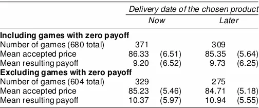
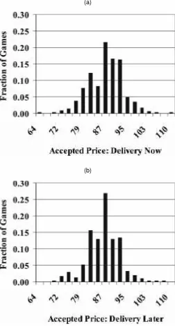
Table 1 contains an overview of the intertemporal choices made by subjects. The top part contains data for all 680 games. In 371 games subjects chose a product with instant delivery (corresponding to an instant payoff), and in 309 games sub-jects chose a product with delayed delivery (corresponding to a payoff in 14 days). On average, accepted prices are higher, and the resulting payoffs lower, for chosen products with in-stant delivery. This is consistent with the notion that at least some of our subjects discount future payments. Discounting is also suggested by Figure 1, which shows the distributions of ac-cepted prices for both delivery dates. Figure 1(a), which shows the distribution of prices for widgets with immediate delivery, has more mass at higher prices than Figure 1(b), which shows the distribution of accepted prices for widgets with delayed de-livery.
Our rst approach to drawing inferences about subjects’ dis-count rates, which can be viewed as revealed intertemporal
Table 1. Accepted Prices and Corresponding Payoffs
Delivery date of the chosen product
Now Later
Including games with zero payoff
Number of games (680 total) 371 309 Mean accepted price 86.33 (6.51) 85.35 (5.64) Mean resulting payoff 9.20 (6.52) 9.73 (6.25)
Excluding games with zero payoff
Number of games (604 total) 329 275 Mean accepted price 85.23 (5.46) 84.71 (5.18) Mean resulting payoff 10.37 (5.97) 10.94 (5.55)
NOTE: Standard deviations are in parentheses.
(a)
(b)
Figure 1. Distribution of Accepted Prices. (a) Prices accepted by sub-jects for immediate-delivery widgets. (b) Prices accepted by subsub-jects for delayed-delivery widgets. Accepted prices higher than 100 imply a loss, because the widget is valued at 100; prices lower than 100 might also imply a loss, depending on accumulated search cost. In the case of a loss, actual payoffs were restricted to 0.
preferenceanalysis, requires only the assumption that subjects prefer higher payoffs to lower payoffs (and the assumption of risk neutrality that we maintain throughout). With this assump-tion, we can derive bounds on each subject’s discount rate by observing their location choices. For example, suppose that a subject stops searching, and his or her best payoffs are 88 for immediate-delivery and 90 for delayed-delivery widgets. If the subject chooses the location that offers immediate delivery, then it follows that his or her discount rate can be no larger than 88/90, whereas if he or she chooses the location offering de-layed delivery, then his or her discount rate can be no smaller than 88/90. This fact allows us to construct bounds on a
sub-Table 2. Combinations of Payoffs for Accepted and Best Alternative Prices
The payoff associated with the best price available for a product with the alternative delivery date is
Delivery date of the chosen product
Now Later
Higher than the payoff for the chosen product
Case 1 109 games
Case 4 92 games Equal to the payoff for the
chosen product
Case 2 3 games
Case 5 4 games Less than the payoff for
the chosen product
Case 3 217 games
Case 6 179 games
NOTE: Game counts exclude cases where the payoff is zero.
ject’s discount rate, given that the subject has a meaningful choice between delivery dates. In particular, only those games in which the subject has prices that would result in positive pay-offs at both delivery dates contain information about his or her discount rate. This is the case for 604 of the total 680 games. The bottom part of Table 1 provides descriptive statistics for the sample that excludes the 76 zero-payoff games from the re-vealed preference analysis.
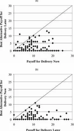
Table 2 lists the six situations that a subject can face when he or she decides to stop searching. These situations are dened by comparing payoffs for the chosen delivery date with the payoffs corresponding to the best price available at the alternative de-livery date (of which many will be zero as well). Observations for cases 1, 2, and 3 (delivery now) are shown in Figure 2(a); observations for cases 4, 5, and 6 (delivery later) are shown in Figure 2(b). Observations that correspond to cases 1 and 4 are above the 45-degree line, observations that correspond to cases 2 and 5 are on the 45-degree line, and observations that correspond to cases 3 and 6 are below the 45-degree line. Ta-ble 2 also contains the counts of these observations.
From these observed decisions on intertemporal tradeoffs, we can compute bounds on subjects’ discount rates. We ex-clude those cases in which subjects chose combinations of price and date that were strictly dominated in terms of the associated payoffs (e.g., all case 4 observations) and all observations with zero payoff for the best available price at the alternative delivery date.
We end up with observed choices that allow us to obtain lower and/or upper bounds that lie in the [0;1] interval for many of our subjects. Because all subjects play 10 games, we have more than one lower or upper bound for some subjects. In these cases, we compute the intrasubject maximum of the lower bound for the former, or the intrasubject minimum of the upper bound for the latter. There were several cases in which a subject’s decisions did not reveal an upper or a lower bound. In these cases we set the lower bound to 0 and/or the upper bound to 1. Once these bounds were determined, we computed the “re-vealed preference” estimate of the subjective discount rate for all subjects as the mean of the lower and upper bounds.
Our revealed preference estimation procedure can be inter-preted as follows. We rst impose a uniform distribution over the [0;1] interval as a prior for the subjective discount rate. In particular, we rule out the possibility that the discount rates can be above 1 or below 0. Observed lower bounds above zero and upper bounds below 1 allow us to narrow the prior. For those subjects for whom we cannot construct bounds away from
(a)
(b)
Figure 2. Payoffs Resulting From the Accepted Price (horizontal axis) Versus Payoffs That Would Result From the Best Price at the Alternative Delivery Date (vertical axis). (a) Prices accepted by sub-jects for immediate-delivery widgets. (b) Prices accepted by subsub-jects for delayed-delivery widgets. In both panels the diamonds represent the trade-off between prices for widgets delivered at two different points in time; therefore, they provide relative prices across time and can be used to bound discount rates. In (b), diamonds above the 45-degree line rep-resent inconsistent choices, because the payoff associated with the ac-cepted price for delayed-deliverywidgets is lower than the potential pay-off that would result from the best available price for immediate-delivery widgets.
0 and 1, we obtain an estimate of .5. (This is the case for 31 sub-jects.) Note that using the mean of the set of possible discount rates as our point estimate is arbitrary, and this choice is made mainly for convenience.Moreover, this is not a central aspect of our analysis. Our primary interest is in whether differences ap-pear between approaches, and we use this estimate within each inferential approach presented later.
Table 3. Estimates of Subjective Discount Rates Under Various Behavioral Assumptions
Mini- Maxi- Standard Behavioral assumption Mean mum mum deviation
No restriction (revealed preference)
Lower bound .22 0 1.00 .31
Upper bound .97 :25 1.00 .15 Mean of bounds .60 :13 1.00 .18 Optimal behavior .64 0 1.00 .33 Assigned heuristic .70 0 1.00 .22
NOTE: The fth column reports the standard deviation of the cross-sectional distribution of discount rate point estimates. The total number of subjects is 68.
Table 3 summarizes the distribution of the bounds on sub-jective discount rates and the estimates of subsub-jective discount rates that we obtain. In general, the bounds on discount rates are relatively wide, and they contain a fair amount of heterogene-ity; this corresponds to the scattered price observations shown in Figure 2. It is evident that the revealed preference approach without stronger behavioral assumptions does not narrow the at prior substantially.
In the following sections we discuss how imposing additional assumptions on subjects’ behaviors allow us to use the infor-mation generated in our experiment to obtain more precise es-timates of their subjective discount rates. These approaches of-fer a major improvement. Relative to the revealed preof-ference analysis presented in this section, more informative estimates can be obtained when observed behavior in all games is used, instead of behavior only in those games that have nonzero pay-offs and a valid intertemporal trade-off (a subset that is empty for some subjects).
4. INFERENCE UNDER RATIONAL EXPECTATIONS
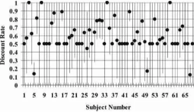
Figure 3 suggests that the revealed intertemporal preference approach provides quite imprecise inference about our subjects’ discount rates. Although it is attractive in that it requires very weak behavioral assumptions, this also means that only the nal decision in each game—the location decision—informs the dis-count rate. Under stronger behavioral assumptions, it is usually the case that continuation decisions inform the discount rate as well. We adopt this approach in this and subsequent sections.
A natural starting point is to assume that subjects follow the rational expectations stopping rule. Under this assumption, the subjective discount rate is identied and can be estimated as the only free parameter of the corresponding decision process. To see this, it is useful to derive the optimal solution to the search task. For the remainder of this article, we label a subject whose behavior is consistent with this rule as a “rational expectations” agent.
Because the value of the widget in the experimental task is 100 tokens, and because each search costs 1 token, it is rea-sonable to derive the solution to the problem under the re-striction that the number of searches cannot exceed 100. Let t2 f1;2; : : : ;100gdenote the number of searches that the ject has made. (For notational convenience, we suppress a sub-ject index as long as no confusion can arise.) After making the tth search the agents’ state vector isStD ft;pb
0;pb1g, wherepb0is the lowest price that the subject has encountered for immediate
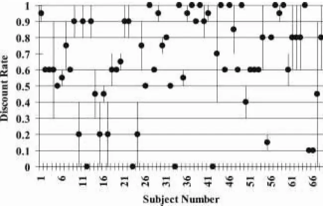
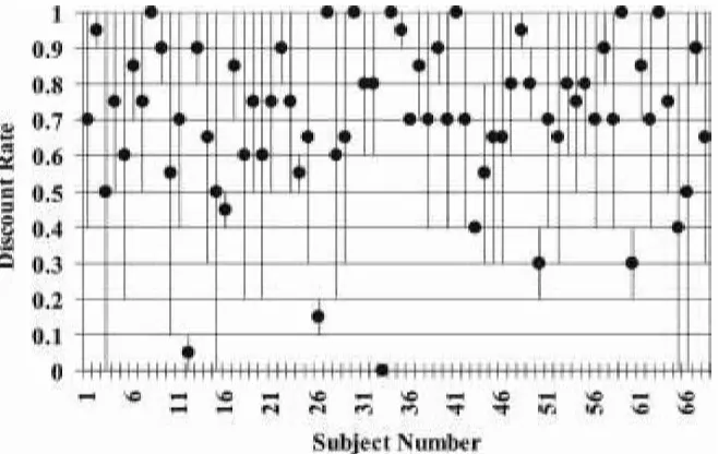
Figure 3. Discount Rate Estimates Obtained With a Revealed Preference Procedure. The revealed preference estimation procedure provides only bounds on individuals’ discount rates. Each vertical line indicates an estimated range of possible discount rates for an individual in our sample. Ranges reect the prior restriction that discount rates must be between 0 and 1. We choose to report the mean of each subject’s estimated range as the point estimate of his or her discount rate (represented as a solid circle). Although behaviorally robust, taking our data to the revealed preference procedure yields wide bounds on the discount rate for most subjects, and does not inform the discount rate at all for 31 of our 68 subjects (their lower bound remains at 0 and their upper bound at 1).
delivery andpb1is the lowest price encountered for delayed de-livery. After thetth search, the agent may either stop searching and choose a location from which to buy the item, or continue to search. After the agent has stopped searching, he or she will buy the item from the location that provides the highest payoff. The available payoffs are
50.St/Dmaxf0;100¡pb0¡tg; 51.St/Dmaxf0; ±.100¡pb1¡t/g;
(1)
where ± is the agent’s rate of time preference. It is conve-nient to dene the chosen payoff, conditional on stopping, as
5.St/Dmax.50.St/; 51.St//. The agent stops searching only if the stopping value is higher than the continuation value. The recursive formulation of this decision problem is, therefore,
Vt.St/Dmaxf5.St/;E[VtC1.StC1/jSt]g; (2) whereErepresents the mathematical expectations operator and the expectation is taken with respect to the distribution of StC1jSt.
It is immediate from (1) and (2) that this problem has, at every t, the reservation price property. That is, there is some best available price for immediate-delivery items such that at this and any lower price, it is optimal to stop searching, whereas at every higher best available price, it is optimal to continue searching. This reservation price depends both on the number of completed searches and on the best available price for delayed-delivery items. To see this, note that both arguments that en-ter the maximization operator in (2) are weakly decreasing (in both prices). When prices are sufciently low, the continuation value is equal to the stopping payoff less 1. At sufciently high prices, the stopping payoff is 0, whereas the continuationpayoff is necessarily bounded above 0 (because all price draws are in-dependent,and the measure of prices that generate positive pay-offs is strictly positive). The intermediate value theorem then implies that the stopping and continuation value cross at least
once. That this crossing is unique follows from the fact that the slope of the stopping payoff at the crossing point must be¡1 (because the crossing occurs at a positive value for the stopping and continuation payoff), and the slope of the continuationpay-off function is evidently bounded from below by¡1 (because a one-unit improvement generated by the current price draw can never do better than improve the continuation payoff by one unit).
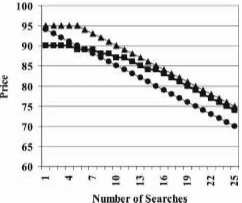
From (1) and (2), it is also easily seen that both reservation prices depend on the rate of time preference,±. One way to see this is simply to observe that the continuation value incor-porates both immediate-delivery and delayed-delivery events, and that the value of delayed delivery clearly depends on the rate of time preference. Figure 4 plots the path of reservation prices, calculated by solving the dynamic discrete choice prob-lem implied by (1) and (2) numerically, for the cases±D1:0 and±D:1. Note that by “reservation price,” we mean that the subject should stop searching if the price draw is less thanor equal tothe reservation value. Note also that we report only integer-valued prices, consistent with the design of our experi-ment.
When the discount rate is unity, the problem reduces to stan-dard search with recall with a single reservation price. This reservation price begins at 90, decays slowly to about 87 by round 10, reaches 80 by the 19th search, and decays at a rate of about 1 per round from that point forward. When the dis-count rate is .1, the reservation price for the current payoff fol-lows roughly the same pattern as the earlier case, but is slightly higher. The reason is that the continuation value falls with the discount rate, so the person is willing to accept smaller stop-ping payoffs. Reservation prices for delayed delivery follow an inverted U-shaped pattern. The very low initial values arise be-cause the continuation value incorporates the chance of nd-ing an item for immediate delivery, and offsettnd-ing this expected value under heavy time discounting requires very low prices for delayed delivery.
Figure 4. Rational Expectations Reservation Prices for Alternative Discount Rates and Delivery Dates. The three curves describe the high-est integer price that a subject with rational expectations would pay for a widget, by cumulative number of search attempts. With a discount rate (delta) of 1, the subject is indifferent between delivery now and delivery later, so there is only one reservation price curve. When the discount rate is less than 1, subjects prefer delivery now to delivery later, all other factors being equal. Because the task is search with recall, to calculate the reservation prices, we assume that the best available price for de-livery at the alternative date is 100. Subjects with discount rates less than 1 are willing to pay slightly more for delivery now than are sub-jects with unit discount rates. Subsub-jects incur a 1-unit cost per search, and their reservation prot level declines with the number of searches. When delta is 1, the reservation prot begins at 9, but declines to 1 by the 15th search. ( ¥ , deltaD1:0; , deltaD0:1, now; N , deltaD0:1, later.)
With reservation prices in hand, it is a simple matter to es-timate the discount rate for each individual. The decision task requires the subject to decide when to stop searching and, once stopped, the location from which to purchase the widget. Given any discount rate, in each period, each state-contingentcontinu-ation decision is either consistent or inconsistent with the reser-vation price associated with that discount rate. When the subject stops searching and chooses a location, that choice is either con-sistent or inconcon-sistent with the given discount rate. Hence ifTj represents the number of locations searched before the subject stopped in gamej, then the subject makesT1C ¢ ¢ ¢ CT10C10 payoff-relevant decisions during the course of the experiment. We associate each subject with the discount rate that is con-sistent with the greatest number of his or her actual decisions. (This procedure is formalized in the next section.)
In this research we consider only 11 discount rate values,
f0; :1; : : : ;1:0g. Such a coarse grid reduces the computational burden, and prior checks conrmed that choices for most sub-jects in our sample are not sensitive to smaller changes in the discount rate. Figure 5 illustrates our discount rate inferences for each subject. The solid circle in the gure represents the point estimate of the discount rate. For 36 of our subjects, the best discount rate is not unique; several discount rates explain the subject’s choices equally well. In these cases the point esti-mate is assumed to be the mean of the candidate values, which is described in the gure by a solid circle in the middle of a line segment. These line segments, therefore, have the same in-terpretation as those reported in the revealed preference analy-sis results. In particular, there is a sense in which a longer line segment implies more uncertainty about a subject’s discount rate, but the line segments do not represent standard errors. (Although we do not report them here, it is straightforward to bootstrap standard errors for the lengths, positions, and, conse-quently, midpoints of the line segments.) The mean of the dis-count rate point estimates is .65, and the median is .68. Overall, the model predicts about 91% of our subjects’ choices.
Figure 5. Estimates of Discount Rates Under Rational Expectations. The procedure for generating these estimates uses the assumption that individuals behave as if they have rational expectations. Each vertical line indicates an estimated range of possible discount rates for an individual in our sample. Ranges reect the prior restriction that discount rates must be between 0 and 1. We choose to report the mean of each subject’s estimated range as the point estimate of his or her discount rate (represented as a solid circle). With the rational expectations procedure, we obtain relatively tight bounds on the discount rate for most subjects, and every subject’s discount rate is informed by his or her experimental data.
5. INFERENCE UNDER HEURISTICS
An alternative to assuming that all subjects use the rational expectations decision rule is to impose the weaker assumption that each subject’s decision rule is a member of a prespecied, nite candidate set of decision rules. This approach, therefore, relaxes the rational expectations assumption and allows differ-ent subjects to use differdiffer-ent decision rules. The candidate set might (and in our case does) include the optimal rational ex-pectations rule.
The intuition for our approach is as follows. If the rules in the candidate set generate different state-contingent decisions for at least one state that occurs with positive probability, then the decision rule used by each subject is asymptotically (in the number of decision problems played by the subject) identied. Moreover, if the choices predicted by the decision rules also depend on an intertemporal trade-off, then it is possible to esti-mate jointly the subject’s subjective discount rate and the deci-sion rule he or she uses. The primary advantage of this proce-dure is that inferences about discount rates are less likely to be biased by misspecication of the decision rule.
5.1 Specication of the Set of Admissible Heuristics
Following the approach taken in earlier experimental work on behavior in search tasks by Hey (1982) and Moon and
Martin (1990), and in a slightly different context by Müller (2001), we base our analysis on a prespecied set of candidate decision rules. We assume in our statistical analysis that sub-jects use one of these rules to determine their stopping decision in every round of the search problem, conditionalon observable state variables and unobservable preference parameters. (In our case, these are the discount rate and, possibly, parameters of the decision rules themselves.)
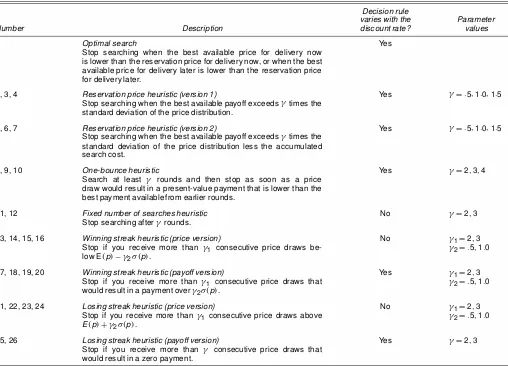
The decision rules we consider fall into three broad classes. The rst class is the solution to the search problem derived un-der rational expectations (rule 1). The second class comprises six sophisticated heuristics that reect some properties of the optimal solution but are still simple to apply (rules 2–7). The third class consists of 19 naive heuristics that are not directly related to the optimal solution but are extremely simple to ap-ply (rules 8–26). Table 4 contains an overview of all 26 rules.
Decision rule 1 is theoptimal search rule. Subjects who fol-low this rule stop searching if the best available price for deliv-ery now is smaller than the reservation price for delivdeliv-ery now, or if the best available price for delivery later is smaller than the reservation price for delivery later. The reservation prices are given by the solution to the search problem under rational expectations, as discussed earlier in Section 4.
The next class of decision rules is sophisticated heuristics, which have the reservation price property. We designed these
Table 4. Candidate Decision Rules for the Sequential Search Problem
Decision rule
varies with the Parameter
Number Description discount rate? values
1 Optimal search
Stop searching when the best available price for delivery now is lower than the reservation price for delivery now, or when the best available price for delivery later is lower than the reservation price for delivery later.
Yes
2, 3, 4 Reservation price heuristic (version 1)
Stop searching when the best available payoff exceeds° times the standard deviation of the price distribution.
Yes °D:5;1:0;1:5
5, 6, 7 Reservation price heuristic (version 2)
Stop searching when the best available payoff exceeds° times the standard deviation of the price distribution less the accumulated search cost.
Yes °D:5;1:0;1:5
8, 9, 10 One-bounce heuristic
Search at least ° rounds and then stop as soon as a price draw would result in a present-value payment that is lower than the best payment available from earlier rounds.
Yes °D2;3;4
11, 12 Fixed number of searches heuristic Stop searching after°rounds.
No °D2;3
13, 14, 15, 16 Winning streak heuristic (price version)
Stop if you receive more than °1 consecutive price draws be-low E.p/¡°2¾ .p/.
No °1D2;3
°2D:5;1:0
17, 18, 19, 20 Winning streak heuristic (payoff version)
Stop if you receive more than °1 consecutive price draws that would result in a payment over°2¾ .p/.
Yes °1D2;3
°2D:5;1:0
21, 22, 23, 24 Losing streak heuristic (price version)
Stop if you receive more than°1 consecutive price draws above E.p/C°2¾ .p/.
No °1D2;3
°2D:5;1:0
25, 26 Losing streak heuristic (payoff version)
Stop if you receive more than ° consecutive price draws that would result in a zero payment.
Yes °D2;3
NOTE: We assume that after stopping according to one of these decision rules, subjects accept the price that results in the greatest present-value payment.
rules to take into account two important determinants of the optimal reservation price: the known standard deviation of the price distribution and the accumulated search cost. Subjects who use one of these heuristics stop searching when the best available present-value payment exceeds a certain threshold level. In the rst version (rules 2, 3, and 4), this threshold is a multiple (.5, 1.0, or 1.5) of the standard deviation of the price distribution; note that this threshold is constant over time. In contrast, in the second version we assume that the threshold falls linearly in the accumulated search cost (rules 5, 6, and 7). In that version, subjects always stop after a maximum number of searches. (Because the standard deviation of the price distri-bution is 10, this happens in round 5, 10, or 15, depending on the threshold parameter.)
An intuitive interpretation of these heuristics is that subjects understand that a good realization of the random price process is a price that is well below the mean of the known distribu-tion, and natural focal points for the distance between a price draw and the mean of the distribution are multiples of the stan-dard deviation. Following these sophisticated heuristics does not require solving the underlying dynamic decision problem. In particular, subjects do not form expectationsover future price draws.
Figures 6 and 7 compare the reservation prices for various de-cision rules, discount rates, and delivery dates. Figure 6 shows reservation prices for items with immediate availability implied by rules 2 and 5 (i.e.,° D:5) and a discount rate of 1.0 to the correspondingoptimal reservation price path. The path of rule 2
Figure 6. Reservation Prices for Immediate Delivery Under Ratio-nal Expectations and Heuristic Decision Rules. The curves describe the highest integer price that a subject would pay for an immediately deliv-ered widget for three different decision rules and by cumulative number of search attempts. The rational expectations reservation prices assume a discount rate of unity, and were calculated as described in the legend of Figure 4. The three proles are different. A necessary and sufcient condition for separate (asymptotic) identication of decision rules is that they have different reservation price proles. Table 5 shows a sense in which heuristics 2 and 5 t the data better than the rational expecta-tions rule. A reason is that these heuristics imply relatively high reserva-tion prices, and this is consistent with most subjects’ decisions to stop searching earlier than rational expectations predicts. ( ¥ , rational ex-pectations, , heuristic No. 2; N , heuristic No. 5.)
begins above the optimal path, is about the same at round 5 and then falls and stays below. Hence, relative to the rational expec-tations, following this rule would see subjects either stopping too easily in early rounds or continuing their search when they should stop in later rounds. Rule 5, on the other hand, raises the reservation price at all search durations. Under rule 5, searchers stop with any positive payoff beginning in round 5, whereas un-der the optimal rule this does not occur until about round 20. Figure 7 provides a similar comparison for delayed delivery reservation prices under a discount rate of .5. The reservation price rules are qualitatively similar.
Decision rules 8–12 were suggested by Moon and Martin (1990), following earlier work by Hey (1982). Subjects who follow rule 8, 9, or 10, theone-bounce rule, search at least two, three, or four rounds, respectively, and then stop as soon as a price draw results in a present-value payment that is lower than the best payment available from earlier rounds. Rules 11 and 12 are even simpler; subjects just do axed number of searches (two or three, respectively) and then take the best available price. These rules were designed for an environment with un-known price distributions.
The remaining decision rules are based onwinning streaks (rules 13–20) andlosing streaks(rules 21–26). Subjects who follow these rules stop searching if they receive two or three consecutive price draws that are above or below some xed threshold level. Both winning and losing streak heuristics are formulated in two versions that differ in how these threshold levels are constructed. The rst version is based on the price draws themselves, whereas the second version is based on the present-value payments implied by the current price draw. The threshold levels are, once again, formulated as multiples (.5 or 1.0) of the standard deviation, which we interpret as focal points; details are given in Table 4. All rules based on win-ning or losing streaks take into account knowledge of the price
Figure 7. Reservation Prices for Delayed Delivery Under Rational Expectations and Heuristic Decision Rules. The discount factor used to derive these reservation price proles is .5, and the rational expectations prole was calculated as detailed in the legend of Figure 4. The shape of the reservation price prole is inuenced by the discount rate. This is the source of discount rate identication. ( ¥ , rational expectations;
, heuristic No. 2; N , heuristic No. 5.)
distribution—the idea is that subjects use the standard deviation to determine whether a draw is good or bad. However, subjects who follow these rules falsely assume, at least implicitly, that there is some dependence in the price process. That subjects might use these streak-based rules in search situations such as that of our experiment can be motivated by results from psy-chological research on behavior in uncertain environments (see Rabin 2002).
5.2 Statistical Classication Procedure
Our approach to drawing joint inferences about preferences and heuristics is to determine for each subject the number of choices consistent with each possible combination of decision rule and discount rate, and then choose that which best ts the subject’s behavior. The drawback of this procedure is that it can lead to overtting. The number of decision rules assigned to subjects is unrestricted, and, at least in principle, each subject could be assigned his or her own decision rule (which would not be particularly interesting). An alternative approach, the one that we pursue in this section, is to assign the heuristics from a subset of the universe of possible heuristics and to allow this subset also to be determined by the statistical procedure. To determine jointly the subset of assigned heuristic and each sub-ject’s heuristic and discount rate assignment, we nest the maxi-mum likelihood classication algorithm proposed by El-Gamal and Grether (1995) within a discount-rate grid search.
To implement the El-Gamal and Grether (1995) procedure, we assume that each subject follows exactly one of the heuris-tics in our universe of heurisheuris-tics, and that he or she uses the same heuristic to play every game. (For an alternative approach that does not require specication of the universe of alterna-tives, see Houser, Keane, and McCabe 2002.) This seems rea-sonable in view of the fact that all subjects are experienced when they begin the payoff-relevant games. Of course, a sub-ject’s behavior need not necessarily be perfectly consistent with any of the heuristics in our universe of alternatives. Following El-Gamal and Grether (1995), we circumvent this problem by assuming that subjects play their heuristic with error, and that the error rate is the same across all subjects.
More formally, to implement the classication procedure, we assume that each subject has a xed subjective discount rate,
±i2[0;1]. We also assume that each subject follows a single decision rule,ci2C, whereCis a prespecied universe of can-didate heuristics. Finally, we assume that a subject plays his or her decision rule with error rate, ", and that this error rate is constant over time and across subjects.
Each heuristic/discount rate combination that we consider provides a unique map from a subjecti’s state (information set), Sit, to their continuation decision,dit2 f0;1g. Letd¤
itdenote the observed decision of subjectiin periodt, and letdci;±i
it .Sit/be the unique decision implied by heuristicci and discount rate ±i under informationSit. Then dene the indicator function, xci;±i subjecti’stth continuation decision agrees with the prediction, and 0 otherwise. No difculty arises if an error leads a sub-ject to continue his or her search when he or she should have stopped, because the subject’s state and corresponding continu-ation decision remain dened in subsequent periods. Thus it is
not inconsistent to assume that a subject who violates his or her decision rule in one period can still act according to this rule during the remaining search periods.
Finally, the last decision that a subject makes in every game is the location decision. We assume that the location decision is independent of the continuation decisions and is made with identical error rate. In particular, we assume that a subject who stops with J location alternatives chooses the location given by some candidate decision rule with probability.1¡"/and a member of the set of other possible locations with probabil-ity", independent ofJ.
We observeTi decisions for subjecti. Following El-Gamal and Grether (1995), dene the sufcient statistic Xci;±i
i D
PTi
tD1x
ci;±i
it .Sit/. Then the likelihood function for subjectiis
fci;±i;"¡xci;±i
If there areI subjects, each indexed byi, then a natural way to estimate jointly the discount rate for each subject and their heuristicciis to apply maximum likelihood using
¡ the error rate is assumed to be identical for all subjects.
To avoid overtting with respect to the number of heuris-tics, El-Gamal and Grether (1995) suggested that if there are k heuristics in the set C used to explain all of the subjects’ decisions, then the log-likelihood should be penalized by an amountR.k/. Adopting their suggestion for our environment implies a penalty factor of
R.k/Dklog.2/¡68 log.k/¡klog.26/: (5)
Log-likelihood(4), minus penalty factor (5), is maximized over the set of all possible k-tuples (kD1; : : : ;26) that can be formed from our universe of 26 decision rules.
El-Gamal and Grether (1995) suggested the penalty factor given by (5) for the following reason. LetCk denote a set ofk heuristics. The penalized log-likelihood implied by (4) and (5) is the Bayesian posterior that arises under the priors that (a) the probability that the population includes exactlyk heuristics is 1=2k, (b) all possiblek-tuples of heuristics in anyCkare equally likely (in our case, each has probability 1=26k), (c) all alloca-tions of heuristics to subjects are equally likely (in our case, each has probability 1=k68) and (d) all error rates (between 0 and 1) are equally likely and do not depend on the number of rules used in the population or on the way in which those rules are assigned.
It is worthwhile to point out that an alternative approach for classifying subjects according to their decision rules is based on the EM algorithm (for an application in this context, see Little and Rubin 1983). As discussed by El-Gamal and Grether (1995, sec. 6), using an EM classication algorithm has two advan-tages over our approach. First, because we classify each subject to the rule that maximizes his or her contribution to the likeli-hood function, we are in essence minimizing the number of er-rors attributed to each subject. This results in a downward bias in our estimate of the error rate. Second, small-sample misclas-sication errors are not taken into account when we estimate the
Table 5. Fraction of Correctly Explained Choices by Discount Rate (Means Across Subjects)
Assumed value of the discount rate
Heuristic 1 .9 .8 .7 .6 .5 .4 .3 .2 .1 0
1 (5) .86 .87 .87 .87 .88 .87 .86 .85 .85 .85 .85 2 (21) .95 .95 .95 .94 .94 .93 .92 .90 .90 .89 .89 3 .91 .90 .89 .89 .88 .87 .87 .87 .86 .86 .86 4 .87 .86 .86 .85 .85 .85 .85 .85 .84 .84 .84 5 (46) .96 .96 .96 .96 .95 .95 .95 .94 .93 .92 .92 6 (29) .95 .95 .94 .94 .93 .92 .91 .91 .90 .90 .89 7 (4) .90 .89 .88 .88 .87 .87 .87 .86 .86 .86 .86 8 .46 .46 .46 .46 .45 .46 .46 .46 .47 .50 .58 9 .51 .51 .51 .51 .51 .51 .51 .51 .52 .55 .62 10 .55 .55 .55 .55 .55 .55 .55 .56 .56 .58 .65 11 .41 .41 .41 .40 .40 .40 .40 .40 .40 .39 .39 12 .48 .48 .48 .48 .48 .48 .48 .47 .47 .47 .47 13 .83 .83 .83 .82 .82 .82 .82 .82 .82 .81 .81 14 .83 .83 .83 .82 .82 .82 .82 .82 .82 .81 .81 15 .84 .83 .83 .83 .83 .83 .83 .83 .83 .82 .82 16 .84 .83 .83 .83 .83 .83 .83 .83 .83 .82 .82 17 .84 .84 .84 .84 .83 .83 .83 .83 .83 .82 .82 18 .84 .84 .84 .84 .83 .83 .83 .83 .83 .82 .82 19 .84 .84 .83 .83 .83 .83 .83 .83 .83 .82 .82 20 .84 .84 .83 .83 .83 .83 .83 .83 .83 .82 .82 21 .79 .79 .79 .79 .79 .78 .78 .78 .78 .78 .78 22 .79 .79 .79 .79 .79 .78 .78 .78 .78 .78 .78 23 .82 .82 .82 .82 .82 .82 .82 .82 .82 .81 .81 24 .82 .82 .82 .82 .82 .82 .82 .82 .82 .81 .81 25 .47 .47 .47 .47 .47 .47 .46 .46 .46 .46 .46 26 .47 .47 .47 .47 .47 .47 .46 .46 .46 .46 .46
NOTE: Numbers in parentheses indicate the number of subjects for whom the heuristic is a “best” heuristic. Absence of a number in parentheses indicates that the heuristic is not assigned to any subject. The sum of the assignments is greater than the number of subjects, because some subjects are assigned multiple heuristics.
discount rate. However, as the number of observations per sub-ject tends to innity, both estimation algorithms will coincide with probability 1 and share the same consistency properties (El-Gamal and Grether 1995, p. 1144).
5.3 Inference About Discount Rates
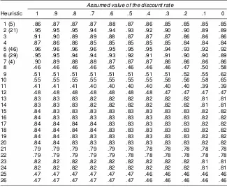
Table 5 reports the aggregate fraction of choices that are con-sistent with each heuristic for each discount rate inf0; :1; : : : ;
1:0g. The numbers of the heuristics are dened in Table 4. For example, in Table 5 the entry of .86 for heuristic 1 and dis-count rate 1 means that a model in which everyone follows ra-tional expectations and has a discount rate of 1 predicts 86% of subjects’ choices. Heuristics 13–26 are streak-based and pro-vide a relatively poor and relatively discount rate–insensitive t. The worst ts are provided by heuristics 22–26, the one-bounce and xed search heuristics. Recall that the latter heuris-tics have been designed for search tasks in which the distrib-ution of prices is unknown, so it is not surprising that in our experiment they are dominated by heuristics that account for knowledge of the price distribution. The best aggregate ts are provided by the six reservation price heuristics (rules 2–6) and the optimal, rational expectationsbehavior (rule 1). That the op-timal rule is consistent with up to 88% of all choices is in line with ndings reported in earlier literature that behavior is often nearly optimal in search experiments (see Sec. 1).
Although behavior is nearly optimal, it is clear that the reser-vation price heuristics provide a superior aggregate t. Heuris-tic 5, reservation price proles for which are plotted in Figures 6 and 7, matches 96% of all choices made in the experiment when the discount rate is above .6. Note also that although aggregate consistency tends to be higher at higher discount rates for the
reservation price heuristics, it is highest for the optimal rule when the discount rate is .6. This suggests that subjects are, on average, stopping to search sooner than is consistent with ratio-nal behavior at high discount rates. Although reducing the dis-count rate helps to t stopping decisions when a current payoff is chosen, it becomes inconsistent with the decision to accept a delayed payoff. A relaxed stopping criterion along with a high discount rate, which reconciles the decision to accept delayed payoffs, is consistent with our reservation price heuristics.
Table 5 reports the number of subjects whose behavior is best explained by each heuristic. These counts appear in parenthe-ses next to the heuristic number, unless the heuristic was not assigned to any subject. Five heuristics appear in at least one of the subjects’ best-tting sets: 1, 2, 5, 6, and 7. The reason why the number of heuristic assignments exceeds the number of subjects is that for 24 subjects, multiple heuristics are able to explain their behavior equally and maximally well. (The like-lihood function is at with respect to some decision rules.) Heuristics 2, 5, and 6 occur most frequently; at least one of these appears in all but two subjects’ best-tting sets. Two sub-jects’ choices are uniquely best explained by heuristic 7. The rational expectationsrule is assigned to ve subjects, but always in conjunction with a sophisticated heuristic. Hence, although observed behavior is consistent with optimal, rational expecta-tions behavior in ve cases, it is also consistent with decisions based on some heuristic that is much easier to use.
Turning now to estimation results, Figure 8 summarizes the outcome of the El-Gamal and Grether procedure when applied to our data. Each dot corresponds to a single subject. The la-bel above the dot reports the heuristic to which the subject was assigned. In 21 cases there are multiple assignments. For exam-ple, “256” indicates that the subject’s behavior is equally well
Hou
s
er
a
nd
Win
ter
:
Beh
avi
oral
Ass
um
pti
on
s
a
nd
Stru
c
tural
In
fer
en
ce
7
5
Figure 8. Assigned Heuristics and Fit. From an initial universe of 26 heuristics, our statistical procedure, based on that of El-Gamal and Grether (1995), chooses 3 to explain our subjects’ behaviors. The label on each dot represents the heuristic(s) assigned to each subject. The vertical position of each dot represents the fraction of a subject’s choices accurately predicted by the assigned heuristic(s). For example, subject 1 has 97% of his or her choices correctly explained by heuristics 2, 5, and 6 (where the heuristic numbering is as dened in Table 4). The rational expectations heuristic was included in the initial 26 but is not part of the nal set of three. Each of the nal three heuristics is an easily implemented version of a reservation price rule.
Figure 9. Estimates of Discount Rates Under Heuristics. The procedure used to generate these estimates is robust to several types of behavior, as described in Table 4. Each vertical line indicates an estimated range of possible discount rates for an individual in our sample. Ranges reect the prior restriction that discount rates must be between 0 and 1. We choose to report the mean of each subject’s estimated range as the point estimate of his or her discount rate (represented as a solid circle). With this procedure, the discount rate bounds are generally tighter than those generated by the revealed preference analysis, but not as tight as rational expectations based estimates. Three subjects’ data do not inform their discount rate under this procedure.
explained,at potentiallydifferent discount rates, by heuristics 2, 5, and 6. Note that only these three heuristics survive the selec-tion procedure. The vertical posiselec-tion of each dot measures the fraction of choices consistent with that heuristic at an optimal discount rate. This number is not less than 92% for any sub-ject, and for several subjects, all of their choices are predicted by their assigned decision rule(s). Overall, just over 97% of all actual choices are predicted by the best-tting model, implying an error rate of about 5%. This compares to an error rate under the rational expectations restriction of about 18%.
Figure 9 shows inferences about subjects’ subjective dis-count rates. In the cases where multiple heuristics are assigned, the line extends from the lowest to highest discount rate among all of those in the optimal set. For example, if a subject’s be-havior were maximally consistent with rule 5 at discount rates .8 and .9 and also maximally consistent with rule 6 at discount rates .6 and .7, then the line would extend from .6 to .9. As discussed in Section 4, these line segments have an interpreta-tion that is analogous to that reported in the revealed preference estimation results. In particular, longer line segments indicate more uncertainty about an individual’s discount rate. In relation to the inferences drawn from the rational case, estimated dis-count rates are slightly higher on average and clearly less pre-cise. One reason for the reduced precision is that, because con-tinuation value is not incorporated into the reservation prices, variation in the discount rate affects only the reservation price path for delayed-paymentitems. Hence, changes in the discount rate have relatively fewer behavioral implicationsand thus carry less information than in the rational case.
The mean estimated discount rate, where for each subject the estimate is the midpoint of the interval of possible discount rates, is .70 (standard error [SE]D:03) in the present case, as compared with .65 (SED:04) in the rational case. The median is .70, compared with the median of .68 obtained by assuming rational expectations.
At the individual level, the point estimate of the discount rate changes for 56 of 68 subjects when we give up rational expecta-tions restricexpecta-tions in favor of heuristics. It is larger under heuris-tics for 29 subjects, with an average increase of .30, and smaller under heuristics for 27 subjects, with an average decrease of .19. The largest increase in the estimated discount rate is .75 (from 0 under optimal behavior to .75), and the largest decrease is .45 (from 1.0 to .55).
6. EFFECT OF BEHAVIORAL ASSUMPTIONS AT
THE AGGREGATE AND INDIVIDUAL LEVELS
6.1 Effects on Inference About Aggregates
Figure 10 compares the cross-sectional distributions of dis-count rate point estimates that arise under each of the three models considered earlier. These distributions of discount rates could be of interest for policy experiments. For example, whether a particular change in social security payout rules is efcient likely depends on this distribution.
The means of the distributions of point estimates that arise under rational expectationsand heuristic behavior are .65 (SED
:04) and .70 (SED:03). A two-sample, two-tailedt test for equality of means cannot reject the null that the means of these distributions are the same at standard signicance lev-els (pD:26). A two-sample Wilcoxon rank-sum test cannot reject the null that the medians of these two distributions are the same (pD:54). A Kolomogorov–Smirnov cannot reject the null that the rational expectations and heuristic-based distribu-tions of discount rates’ point estimates (across subjects in our sample) are the same at the 5% signicance level (pD:07). Moreover, the mean of the revealed preference estimates, .59 (SED:20), is not statistically different from the mean of the ra-tional expectations discount rate distribution. However, the me-dian (.50) and overall distribution both differ signicantly from
Figure 10. Cross-Sectional Density of Discount Rate Point Estimates Under Alternative Behavioral Assumptions. The white, tan, and black bars correspond to estimates generated by revealed preference, heuris-tics, and rational expectations procedures. The height of each bar indi-cates the number of subjects assigned to the bar’s corresponding dis-count rate. For example, 38 of our subjects were assigned a disdis-count rate of .5 in the revealed preference analysis. Inference with respect to the central tendency of the cross-sectional discount rate distribution, which might be of particular interest to policy analysts, is not statis-tically signicantly different in the rational expectations and heuristics cases. Moreover, the heuristics-based and rational expectations–based distributions of discount rate estimates are not statistically signicantly different.
the others. Thep values associated with thet test, rank-sum test, and Kolomogorov–Smirnov test are .17, .01 and 0 against the distribution obtained assuming rational expectations and 0, 0, and 0 against the distribution obtained under the heuristics assumption.
These ndings suggest that when a researcher wants to es-timate the central tendency of the cross-sectional distribution of discount rates, there is little cost entailed in imposing ratio-nal expectations instead of using a more robust, but in our case cumbersome, heuristics approach. Often, however, an impor-tant additional goal of structural estimation is a policy analysis that depends on functions of the structural parameters. To in-vestigate whether policy analysis might be affected by differ-ent behavioral assumptions, we examine how inferences about the price elasticity of demand for immediately available wid-gets compare under rational expectations and heuristic decision rules.
We begin by simulating the baseline quantity demanded un-der the restriction of rational expectations. Given a discount rate, our simulated search proceeds sequentially with price and availability draws made according to the distributions used in our experiment. Rational expectations is imposed by (a) us-ing the rational expectations stoppus-ing rules and (b) weightus-ing discount rates according to their rational expectations density as described in Figure 10. The high-price simulation proceeds identically to the baseline, except that the location of the price distribution for immediately available widgets is shifted to the right by one unit, becomingN.101;102/, and the rational ex-pectations decision rule is accordingly recalculated for every discount rate. Then the rational expectations price elasticity is determined by comparing the quantity of immediately available widgets purchased in the two simulations in the usual way. The price elasticity under weaker behavioral assumptions is com-puted analogously, with discount rates and heuristics weighted according to their in-sample estimated distribution. In cases where multiple heuristics were assigned to the same subject,
our simulations chose one of the candidates at random. A to-tal of 16 subjects were assigned to heuristic 2; 31 subjects, to heuristic 5; and 21 subjects, to heuristic 6. Hence to com-pute the desired elasticities, we need to obtain four measures of quantity demanded, and to obtain each we conducted 68,000 separate simulations. Specically, we have 68 discount rate– heuristic joint assignments. We simulated under each of these joint assignments 1,000 times.
Under the rational expectations baseline, the immediately available widget accounts for 60% of all purchases in simula-tions with nonzero payoffs. This is higher than the 54% found in the experimental data (see Table 1). Under the high-price sim-ulation, the immediately available widgets are purchased only 55% of the time, suggesting a price elasticity of about 8. Under the heuristics baseline, it turns out that 53% of the widgets pur-chased in games with nonzero payoffs are of immediate avail-ability, and this number falls to about 49% under the high-price simulation, implying a price elasticity of just over 7.
These calculations ignore games with zero payoffs. It is in-teresting to note that in the data, 11% of the games resulted in zero payoffs, whereas in the heuristic and rational expectations simulations these numbers are 7% and 18%. The overall av-erage payoff from rational expectations simulations, under the heuristic discount rate distribution and including zero payoff games, is 1.3% higher than the overall average payoff from the heuristic simulations. If half of the zero payoff games are in-cluded in both the immediate and delayed delivery categories, then the rational expectations elasticity estimate becomes 6.4, whereas while the heuristic elasticity changes to 7.0. Taken to-gether, these results seem to suggest that, at least in our case, elasticity estimates are not very sensitive to the rational expec-tations assumption.
6.2 Validity at the Individual Level
Although the cross-sectional distributions of the discount rate estimates are quite similar, we pointed out earlier that infer-ence about an individual’s discount rate often varies substan-tially with behavioral assumptions. In many cases relevant for policy analysis, particularly those in which interest centers on a proper subset of the sample, it is important to have condence in individual estimates. In this section we show that, in a nar-row sense, the estimates obtained under the weaker assumption of heuristic behavior seem to have greater validity at the in-dividual level than those obtained under rational expectations or by a revealed-preference analysis. Because we cannot know any subject’s true discount rate, our approach to assessing the external validity of our estimation approach is to compare esti-mated discount rates with an independentmeasure of the extent to which one considers future consequences when making de-cisions.
In psychology, several scales dealing with individuals’ at-titudes toward intertemporal trade-offs have been developed. We use the construct of “consideration of future consequences” (CFC), introduced by Strathman, Gleicher, Boninger, and Ed-wards (1994). These authors argued that this construct repre-sents “a stable individual difference in the extent to which peo-ple consider distant versus immediate consequences of poten-tial behaviors” (Strathman, Gleicher, Boninger, and Edwards,