Full Terms & Conditions of access and use can be found at
http://www.tandfonline.com/action/journalInformation?journalCode=ubes20
Download by: [Universitas Maritim Raja Ali Haji] Date: 13 January 2016, At: 00:20
Journal of Business & Economic Statistics
ISSN: 0735-0015 (Print) 1537-2707 (Online) Journal homepage: http://www.tandfonline.com/loi/ubes20
Deviance Information Criterion for Comparing
Stochastic Volatility Models
Andreas Berg, Renate Meyer & Jun Yu
To cite this article: Andreas Berg, Renate Meyer & Jun Yu (2004) Deviance Information
Criterion for Comparing Stochastic Volatility Models, Journal of Business & Economic Statistics, 22:1, 107-120, DOI: 10.1198/073500103288619430
To link to this article: http://dx.doi.org/10.1198/073500103288619430
View supplementary material
Published online: 01 Jan 2012.
Submit your article to this journal
Article views: 215
View related articles
Deviance Information Criterion for Comparing
Stochastic Volatility Models
Andreas B
ERGDepartment of Statistics, University of Auckland, Private Bag 92019, Auckland, New Zealand (andreas@stat.auckland.ac.nz)
Renate M
EYERDepartment of Statistics, University of Auckland, Private Bag 92019, Auckland, New Zealand (meyer@stat.auckland.ac.nz)
Jun Y
UDepartment of Economics, University of Auckland, Private Bag 92019, Auckland, New Zealand (j.yu@auckland.ac.nz)
Bayesian methods have been efcient in estimating parameters of stochastic volatility models for analyz-ing nancial time series. Recent advances made it possible to t stochastic volatility models of increasanalyz-ing complexity, including covariates, leverage effects, jump components, and heavy-tailed distributions. How-ever, a formal model comparison via Bayes factors remains difcult. The main objective of this article is to demonstrate that model selection is more easily performed using the deviance information criterion (DIC). It combines a Bayesian measure of t with a measure of model complexity. We illustrate the per-formance of DIC in discriminating between various different stochastic volatility models using simulated data and daily returns data on the Standard & Poors (S&P) 100 index.
KEY WORDS: Bayesian deviance; Jumps; Leverage effect; Markov chain Monte Carlo; Model com-plexity; Model selection.
1. INTRODUCTION
Progress in Bayesian posterior computation due to Markov chain Monte Carlo (MCMC) methods has made it possible to t increasingly complex statistical models and entailed the wish to determine the best tting model in a potentially huge class of candidates. Thus, it has become more and more important to develop efcient model selection criteria. A recent proposal by Spiegelhalter, Best, Carlin, and van der Linde (2002) was the deviance information criterion (DIC), a Bayesian version or generalization of the well-known Akaike information criterion (AIC) (Akaike 1973), related also to the Bayesian (or Schwarz) information criterion (BIC) (Schwarz 1978). Similar to AIC and BIC, it trades off a measure of model adequacy against a measure of complexity. DIC is easy to calculate and applicable to a wide range of statistical models. It is based on the posterior distribution of the log-likelihood or the deviance, following the original suggestion of Dempster (1974) for model choice in the Bayesian framework. This model comparison criterion has al-ready been applied successfully to complex models in the eld of medical statistics (Zhu and Carlin 2000). In this article, we demonstrate its usefulness in the model selection process for -nancial time series. The aim of this article is, therefore, to intro-duce DIC to the nancial modeling community and show how to use it for the family of stochastic volatility (SV) models.
Indeed, many model-checking criteria (Carlin and Louis 1996; Gelman, Carlin, Stern, and Rubin 1996; Gilks, Richardson, and Spiegelhalter 1996; Key, Pericchi, and Smith 1999) have been proposed and discussed before the develop-ment of DIC. Whereas Bayes factors (e.g., Kass and Raftery 1995) have been viewed for many years as the only correct way to carry out Bayesian model comparison, they have come un-der increasing criticism of late (Kass and Raftery 1995; Lavine
and Schervish 1999). One serious drawback is that they are not well dened when using improper priors, which is typically the case in practice when employing noninformative priors. This
led to modications, such as thepartial Bayes factor(O’Hagan
1991), theintrinsic Bayes factor(Berger and Pericchi 1996),
and thefractional Bayes factor(O’Hagan 1994). These
modi-cations suffer from more or less arbitrary choices of training samples, weights for averaging training samples, and fractions, respectively. For specifying Bayesian stochastic volatility (SV)
models, however, informative and, thus,properprior
distribu-tions are usually employed and Bayes factors are well dened. Nonetheless, the number of unknown parameters in Bayesian SV models is large (exceeding the number of observations) because of the latent volatilities. Calculation of the Bayes factor for comparing any two models requires the marginal likelihoods and, thus, a marginalization over the parameter vectors in each model. If the dimension of the parameter space is large, these implicit, extremely high-dimensionalintegration problems pose a formidable computational challenge. In the context of SV models, Kim, Shephard, and Chib (1998) and Chib, Nardari, and Shephard (2002) showed how to compute Bayes factors using the marginal likelihood approach of Chib (1995) and
eval-uating the marginal likelihood at the posterior mean using
parti-cle ltering(Kitagawa 1996; Pitt and Shephard 1999a; Doucet, de Freitas, and Gordon 2001). Still, it remains a computation-ally intensive task and is not a particularly user-friendly tool for practicing statisticians. In their review of MCMC methods
© 2004 American Statistical Association Journal of Business & Economic Statistics January 2004, Vol. 22, No. 1 DOI 10.1198/073500103288619430
107
for computing Bayes factors, Han and Carlin (2001, p. 29) con-cluded that “all of the methods: : :discussed require substantial time and effort (both human and computer) for a rather mod-est payoff, namely a collection of posterior model probability estimates: : :. As a result, one might conclude that none of the methods herein is appropriate for everyday, ‘rough and ready’ model comparison, and instead search for more computation-ally realistic alternatives.”
A well-known estimate of the marginal likelihood developed by Newton and Raftery (1994) is the harmonic mean of the like-lihood values. It is easy to compute and simulation consistent but not stable because the inverse likelihood does not possess a nite variance (Chib 1995). Other shortcuts to the calcula-tion of Bayes factors that avoid multidimensional integracalcula-tion
through large sample approximationsof¡2 ln(Bayes factor)
in-clude the familiar BIC, also referred to as the Schwarz crite-rion (Schwarz 1978), and the related penalized likelihood ratio model choice criterion, AIC. Either criterion requires the spec-ication of the number of free parameters in each model. If we
consider a nonhierarchical Bayesian model with parameterµ,
a at prior would correspond to a exible and, thus, complex model, whereas a tight prior constrains the model. The classi-cal denition of model complexity as the “number of unknown parameters” could thus be considered as a special case corre-sponding to a noninformative prior. However, for a complex hi-erarchical model the specication of its dimensionality is rather arbitrary. This is typically the case for an SV model, where the
parameters are augmented by thenlatent volatilities, withn
be-ing the sample size. As these are not independent but exhibit a Markovian dependence structure, they cannot be counted as
nadditional free parameters. Thus, neither BIC nor AIC is
ap-plicable for SV model comparison. As detailed in Section 3, DIC avoids this dilemma by using a complexity measure for the effective number of parameters that is based on an information-theoretic argument. This quantity is readily obtained from an MCMC analysis, which makes algebraic forms and large sam-ple approximations obsolete.
It is usually hard to specify prior model probabilities nec-essary for the calculation of posterior model probabilities. By using DIC as a formal approach to model selection, combin-ing a measure of t and complexity, we can avoid this need. However, we caution in general against basing model choice solely on information criteria, as many other factors such as the model’s inherent plausibility and the robustness of its in-ferences and model diagnostics (as, for instance, outlined in Kim et al. 1998, sec. 4.2; Spiegelhalter et al. 2002, sec. 6) need to be taken into account. In many instances, when none of the models is clearly superior, model averaging (Hoeting, Madigan, Raftery, and Volinsky 1999) might be more appropri-ate. Whether DIC can be used as a basis for model averaging is still an open question. And it should also be stressed that no prior model probabilities are necessary for the calculation of Bayes factors.
The outline of the article is as follows: Section 2 gives an introduction to SV models, followed in Section 3 by the de-nition and properties of DIC. Section 4 reviews Chib’s (1995) method for calculating the marginal likelihood based on parti-cle ltering and Newton and Raftery’s (1994) harmonic mean estimate of the marginal likelihood. In Section 5 we present re-sults from a simulation study and compare the model ranking
implied by the marginal likelihood, harmonic mean, and DIC. Section 6 applies DIC to compare the t of various SV models to a dataset previously analyzed in the literature. We also assess the performance of DIC using the Bayes factor as a gold stan-dard and examine the prior sensitivity of DIC. In Section 7 we present our conclusions.
2. THE STOCHASTIC VOLATILITY MODEL
In both the theoretic nance literature on option pricing and the empirical nance literature, the SV model (Taylor 1982; Hull and White 1987) has received much attention in recent years. It has become a powerful alternative to the autoregressive conditional heteroscedasticity (ARCH) and generalized autore-gressive conditionalheteroscedasticity(GARCH) models intro-duced by Engle (1982) and Bollerslev (1986). Ghysels, Harvey, and Renault (1996) and Shephard (1996) gave excellent reviews of the model.
Given a time series of daily returnsfytgntD1, a basic SV model
consists of an observation equation
ytjhtDexp.ht=2/ut; tD1; : : : ;n; (1)
that describes the distribution of the data given unknown states, the log-volatilitiesht, and a state equation
htjht¡1D¹CÁ.ht¡1¡¹/Cvt; tD1; : : : ;n; (2)
which models the day-to-day variation of the volatilities as a
Markov process. Here yt is the response variable, ht is the
log-volatility process, and the errorsutandvtare uncorrelated
Gaussian sequences withut»N.0;1/andvt»N.0; ¿2/. We
collect the three model parameters in a vectorzD.Á; ¹; ¿2/. In Sections 5 and 6 we will introduce extensions of the basic model to more complex SV models. An example of such an extension is the inclusion of a level effect in the observation equation, namely,
ytDx°t exp.ht=2/ut; tD1; : : : ;n;
where xt denotes a time-varying covariate. The parameter°
plays an important role in analyzing interest rate data (for de-tails refer, e.g., to Chan, Karolyi, Longstaff, and Sanders 1992; Brenner, Harjes, and Kroner 1996). In other applications, for example, stock market data, it is common to set this parameter equal to 0 (see Sec. 5).
Classical parameter estimation for this model is extremely difcult, because of the nonanalytic form of the likelihood function. Harvey, Ruiz, and Shephard (1994) employed a quasi-maximum likelihood technique, whereas Sandmann and Koopman (1998) used the maximum likelihood Monte Carlo method. Several method-of-moment approaches such as the efcient method of moments (Gallant and Tauchen 1996; Andersen, Chung, and Sørensen 1999), the spectral method of moments (Singleton 2001; Chacko and Viceira 2003; Knight, Satchell, and Yu 2002), the simulated method of moments (Dufe and Singleton 1993) and the generalized method of moments (Melino and Turnbull 1990; Andersen and Sørensen 1996) have also been used to estimate the model parameters.
Whereas some of the previously mentioned techniques use ad hoc criteria (see Andersen et al. 1999 for a review and com-parison of various estimation techniques for the SV model),
a Bayesian approach is based on a sound statistical paradigm. Bayesian posterior computations are performed using MCMC techniques. Several different algorithms have been proposed by Jacquier, Polson, and Rossi (1994) and Kim et al. (1998) and further developed in Chib et al. (2002). Although more efcient updating techniques for SV models exist, we employ the all-purpose Bayesian software package BUGS based on the single-update Gibbs sampler as described in Meyer and Yu (2000) for ease of implementation. The SV model is a typical example of a hierarchical model, in which the number of unknowns, that is, the parameters (z) and the unknown states (h1; : : : ;hn),
ex-ceeds the number of observations. The number of free parame-ters in the model could be the number of model parameparame-ters (3) or the number of states plus the number of model parameters
.nC3/ or something in between. In any case this number is
not well dened and, thus, precludes the use of AIC or BIC for model comparison. We will show that DIC provides an efcient and straightforward approach to dening the effective number of parameters and to identifying the most appropriate model.
3. THE DEVIANCE INFORMATION CRITERION
Assume, in general, that the distribution of the data, yD
.y1; : : : ;yn/, depends on a p-dimensional parameter vectorµ.
(In the context of an SV model,µ encompasses the
parame-ter vectorzand the vector of log-volatilitiesh1; : : : ;hn.) From
a frequentist point of view, model assessment is based on the deviance, the difference in the log-likelihoods between the t-ted and the saturat-ted model. The saturat-ted model refers to the model with as many parameters as observations, which yields a perfect t to the data. By analogy, Dempster (1974) suggested examining the posterior distribution of the classical deviance dened by
D.µ /D ¡2 lnf.yjµ /C2 lng.y/ (3)
for Bayesian model selection. Here f.yjµ / is the likelihood
function, that is, the conditional joint probability density func-tion of the observafunc-tions given the unknown parameters, and
lng.y/ denotes a fully specied standardizing term that is a
function of the data alone [in our applications in Secs. 5 and 6,
g.y/D1]. Dempster (1974) proposed comparing plots and
po-tential summaries such as the posterior mean of D.µ /, and
Spiegelhalter et al. (2002) followed these suggestions in the de-velopment of DIC as a model choice criterion. Based on the posterior distribution ofD.µ /, DIC consists of two components, a term that measures goodness of t and a penalty term for in-creasing model complexity:
DICD NDCpD: (4)
1. The rst term, a Bayesian measure of model t, is dened as the posterior expectation of the deviance
N
DDEµjy[D.µ /]DEµjy[¡2 lnf.yjµ /]: (5)
The “better” the model ts the data, the larger are the
val-ues for the likelihood.D, which is dened asN ¡2 times
log-likelihood, therefore, attains smaller values for “bet-ter” models.
2. The second component measures the complexity of the
model by theeffective number of parameters,pD, dened
as the difference between the posterior mean of the
de-viance and the dede-viance evaluated at the posterior meanµN
of the parameters:
pDD ND¡D.µ /N DEµjy[D.µ /]¡D.Eµjy[µ]/
(6)
DEµjy[¡2 lnf.yjµ /]C2 lnf.yj Nµ /:
By dening¡2 lnf.yjµ /as the residual information in the
datayconditional on µ and interpreting it as a measure
of uncertainty, (6) shows thatpD can be regarded as the
expected excess of the true over the estimated residual
in-formation in datayconditional onµ. This means we can
interpretpDas the expected reduction in uncertainty due
to estimation.
Rearranging (6), one getsDN DD.µ /N CpD. Thus, the DIC
de-ned in (4) can be reexpressed as
DICDD.µ /N C2pD; (7)
which can be interpreted as a classical “plug-in” measure of t plus a measure of complexity. Therefore, the Bayesian measure of tDNDD.µ /N Cpdalready includes a penalty term for model
complexity and could thus be better thought of as a measure of “model adequacy” rather than pure goodness of t.
Spiegelhalter et al. (2002) gave an asymptotic justication of
DIC in the case where the number of observationsngrows with
respect to the number of parameters pand where the prior is
nonhierarchical and completely specied (i.e., without hyper-parameters). In this situation AICDD.µ /O C2p, whereµO de-notes the maximum likelihood (ML) estimate. This is the same
formula as (7) but with the posterior mean µN substituted by
the ML estimateµO. Thus, DIC can be seen as a generalization
of AIC, and it also can be compared to the Schwarz informa-tion criterion BICD ¡2 lnf.yj Oµ /Cplnn. In the special case where the prior is at, a case that corresponds to a frequentist analysis, AIC equals DIC because the ML estimate coincides with the posterior mean. In the context of normal linear regres-sion with uncertainty in the choice of regressors, George and Foster (2001) developed empirical Bayes alternatives to penal-ized likelihood criteria such as AIC and BIC, and Fernandez, Ley, and Steel (2001) pointed out links of Bayes factors with classical information criteria and provided a unifying frame-work.
By applying a logarithmic loss function, Spiegelhalter et al. (2002) gave a decision-theoretic justication for DIC and showed that DIC approximately describes the expected pos-terior loss when adopting a particular model. For additional asymptotic properties ofpDandD, the interested reader is re-N
ferred to Spiegelhalter et al. (2002).
In striking contrast to calculating Bayes factors, computing
DIC via MCMC is almost trivial. An estimate ofDN is easily
cal-culated from the MCMC output by monitoringD.µ /and then
taking the sample mean of the simulated values ofD.µ /. The
effective number of parameterspD can be obtained by
evalu-atingD.µ / at the sample average of the simulated values ofµ
and subtracting this plug-in estimate of the deviance from the estimate ofDN (see also Sec. 5.3).
So far, no efcient method has been developed for calculat-ing reasonably accurate MC standard errors of DIC. Zhu and Carlin (2000) explored this problem, but their approach using the multivariate delta method yields poor results. Their nal recommendation is the “brute force” approach, which is simply
replicating the calculation of DIC someNtimes and estimating
VAR(DIC) by its sample variance
Although this is a painfully time-consuming approach, it at least gives an indication of the inherent variability of DIC.
4. MARGINAL LIKELIHOOD AND HARMONIC MEAN
Because we are going to compare the performance of DIC with that of Chib’s marginal likelihood method and the har-monic mean in the next two sections, it is worthwhile to rst review Chib’s method for calculating the marginal likelihood and Newton and Raftery’s (1994) method for estimating the marginal likelihood by the harmonic mean of the sampled like-lihood values.
4.1 Chib’s Marginal Likelihood
By denition, the marginal likelihoodm.y/is the integral of the likelihood function with respect to the prior density¼.z/:
m.y/D Z
f.yjz/¼.z/dz; (8)
withzdenoting the vector of parameters in the model. As
solv-ing this integral would require high-dimensional integration, Chib (1995) suggested evaluating the marginal likelihood by rearranging Bayes’s theorem
m.y/Df.yjz/¼.z/ ¼.zjy/ ;
where¼.zjy/denotes the posterior probability density function ofz. Thus, the log-marginal likelihood, which is referred to as
lnLin the following, can be calculated by
lnLDlnm.y/Dlnf.yjz/Cln¼.z/¡ln¼.zjy/; (9)
wherezis an appropriately selected high-density point (in this
article we simply use the posterior meanz). The rst term onN
the right side of (9) is the log-likelihood evaluated at the
pos-terior mean of the parameter vectorz (marginalized over the
latent volatilitiesht) and the second term is the log prior
den-sity evaluated at Nz. The third quantity involves the posterior
density, which is only known up to a normality constant. How-ever, an approximation can be obtained by using a multivariate kernel density estimate as suggested in Kim et al. (1998) (see also Silverman 1986, chap. 4), which is based on the posterior
MCMC sample ofz.
We mentioned in Section 2 that the log-likelihood function lnf.yjz/has no analytical form for the SV model as it is mar-ginalized over the latent statesh1; : : : ;hn, and this is why the
exact maximum likelihood method is extremely difcult to im-plement. However, it is possible to approximate the likelihood
by making use of the so-calledparticle ltermethod.
Impor-tant contributions in this area include Gordon, Salmond, and Smith (1993), Kitagawa (1996), and Pitt and Shephard (1999a). By successive conditioning, the log-likelihood lnf.yjNz/can be decomposed into
Taking the latent volatilities into account, each one-step-ahead prediction density has a mixture representation as
f.ytC1jYt;Nz/D
and can, thus, be estimated by
1
In this article we utilize Kitagawa’s algorithm for particle l-tering, which is applicable to a broad class of nonlinear non-Gaussian multidimensional state space models of the form
ytDH.xt;ut/;
(11) xtDF.xt¡1;vt/;
where xt is a k-dimensional state vector (here xtDht is the
one-dimensional log-volatility),vt is an l-dimensional
white-noise sequence with density q.v/, ut is a one-dimensional
white-noise sequence with densityr.u/and assumed
uncorre-lated withfvsgnsD1, andH andF are possibly nonlinear func-tions. LetutDG.yt;xt/and let G0 be the derivative ofG as
a function ofyt. The density of the initial state vector is
as-sumed to bep0.x/. We now summarize all the steps involved in It can be seen that almost all the SV models presented in the next two sections can be rewritten in the state space form (11); hence, it is straightforward to modify the preceding algorithm to t our needs. The only exception is Model 5, which violates
the assumption of no correlation betweenut andvtC1. When
Model 5 is introduced in Section 5, we will show how a sim-ple rewrite of the model allows for a direct use of Kitagawa’s algorithm.
We should point out that more efcient particle lter
algo-rithms are available. An example is theauxiliary particle lter
introduced by Pitt and Shephard (1999a); see the implemen-tation of this particle lter algorithm in Kim et al. (1998), Pitt and Shephard (1999b), Chib, Nardari, and Shephard (1999) and Chib et al. (2002) in the context of SV models. Our experience
suggests that by choosing MD50;000 for Kitagawa’s
algo-rithm one obtains very similar results to the auxiliary particle
lter method withMD2;500.
4.2 Harmonic Mean
Newton and Raftery (1994) suggested the calculation of approximate Bayes factors for model comparison using the har-monic mean of the sampled likelihood values as a
simulation-consistent estimator of the required marginal likelihood. Letµ
denote the parameter vector (augmented by latent volatilities), that is, µD.z;h1; : : : ;hn/, as in Section 3. Similar to (8), the
marginal likelihoodm.y/can be expressed as
m.y/D Z
f.yjµ /f.µ /dµ ;
where f.µ / denotes the joint prior density function ofµ. The
importance sampling method for evaluating this integral is to generate a samplefµ.i/IiD1; : : : ;Mgfrom a so-called
impor-tance sampling densityf¤.µ /. Under quite weak assumptions,
a simulation-consistent estimate ofm.y/is given by
O
asM goes to1, but it does not, in general, satisfy a Gaussian
central limit theorem as 1=f.yjµ /is often not square integrable with respect to the posterior distribution. Thus, a few outlying valuesµ.i/with small likelihood values can have a large effect on the estimate. For this reason Newton and Raftery (1994) also proposed modied estimators that are much more stable than the straight harmonic mean that we used here.
5. A SIMULATION STUDY
The main objective of this simulation study is to see whether DIC is capable of identifying the true model from which the data are generated. Following suggestions by the referees, we also calculate Chib’s marginal likelihood and the har-monic mean estimate for each model within the set of com-peting models. However, we want to point out an argument by
Spiegelhalter et al. (2002, rejoinder) that cautions against us-ing the Bayes factor (or marginal likelihood) as a gold standard against which to assess DIC. The Bayes factor addresses how well the prior has predicted the observed data, whereas DIC ad-dresses how well the posterior might predict future data gener-ated by the same mechanism that gave rise to the observed data. Thus, these criteria cannot, in general, be expected to arrive at the same conclusions as they are designed to answer different questions. Especially for the practical selection of models of nancial time series, we consider this posterior predictive out-look of DIC to be potentially more relevant.
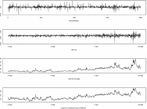
We simulate a dataset comprising 2,000 observations from a stochastic volatility model that includes a jump component as described later. The data are plotted in the rst panel of
Figure 1. This SVCjumps model (Model 6) is very
simi-lar to the one proposed in the simulation analysis by Chib et al. (2002). We use the BUGS (Bayesian Inference Using Gibbs Sampling) software package (Spiegelhalter, Thomas,
Best and Gilks 1996), available online at
http://www.mrc-bsu.cam.ac.uk/bugs/welcome.shtml, for posterior computation. BUGS is an easy-to-learn and easy-to-use Bayesian software package that implements the Gibbs sampler for generating sam-ples from a Markov chain whose equilibrium distribution is the posterior distribution. As demonstrated by Meyer and Yu (2000), it can be applied to t stochastic volatility models. Al-though more efcient Markov chain Monte Carlo techniques exist for tting SV models (Kim et al. 1998), the use of BUGS is highly attractive due to the ease of implementation. In the following, we describe the list of competing models under con-sideration.
5.1 The Models
We t eight different stochastic volatility models to the sim-ulated data, including the true model from which the data are generated (Model 6). For each of the models we list the obser-vation and state equations (fortD1; : : : ;n) and their distribu-tional assumptions. For all cases we assumeut andfvsgnsD1are
uncorrelated unless we claim otherwise. Prior distributions for the unknown parameters are stated in Section 5.2.
Model 1. This model is identical to the basic SV model in Section 2:
Model 2. An additional nonzero mean® is added to the ob-servation equation:
Model 3. An AR(2) process for the state equation:
ytjhtDexp.ht=2/ut; ut
Figure 1. Time Series Plots for Simulated Data, S&P 100, VIX, Logarithm of Absolute Value of S&P 100 Returns.
Model 4. Two independent AR(1) processes as in Harvey et al. (1994), Shephard (1996), Gallant and Tauchen (2001), and Chernov, Gallant, Ghysels, and Tauchen (2003):
ytjhtDexp.¹=2Ch.t1/=2Ch.
2/
t =2/ut;
ut
i:i:d:
» N.0;1/;
h.t1/jh.t¡1/1; Á; ¿2DÁh.t¡1/1Cv.t1/; v.t1/i:»i:d:N.0; ¿2/;
h.t2/jh.t¡2/1; Á2; ¿22DÁ2¢h.t¡2/1Cv
.2/
t ; v
.2/
t
i:i:d:
» N.0; ¿22/:
Model 5. This is Model 1 including a leverage or asymmetric effect by allowing for correlation betweenutandvtC1, that is,
³
ut
vtC1
´
i:i:d:
» N
»³
0 0
´ ;
³
1 ½¿
½¿ ¿2 ´¼
:
This effect is often observed in nancial time series, for exam-ple, in time series of exchange rates and, even stronger, in stock market data. It reveals the market behavior, rst discovered by Black (1976) and described in Engle and Ng (1993).
Although the correlation between ut and vtC1 makes
Kitagawa’s algorithm not directly applicable, a simple rewrite
of this model gives
ytjhtDexp.ht=2/ut; ut
i:i:d:
» N.0;1/;
htjht¡1;yt¡1; ¹; Á; ¿2D¹CÁ .ht¡1¡¹/
C½¿exp.¡:5ht¡1/yt¡1
C¿ q
1¡½2w
t;
where wt
i:i:d:
» N.0;1/and cor.ut;wt/D0. Based on the new
representation, steps 2a and 2b in Kitagawa’s algorithm can be modied by:
2a. GenerateM particles, calledv.tj/,jD1; : : : ;M, from a normal distribution with mean½¿exp.¡:5ht¡1/yt¡1 and variance¿2.1¡½2/.
2b. ObtainMparticles by setting
p.tj/DF¡ft.¡j/1;v.tj/¢; jD1; : : : ;M;
where p.tj/ can be regarded as independent draws from
p.htjyt¡1/.
Model 6. The SVCjumps model includes a jump component and lagged observations in the observation equation:
ytjht;st;qt; ¯D¯yt¡1CstqtCexp.ht=2/ut;
whereqtfollows a Bernoulli distribution that takes a value of 1
with probability·and 0 with probability 1¡·, and ln.1Cst/»
N.¡±2=2; ±2/.
The underlying data are generated from this model using
¹D ¡10,ÁD:96,¿D:345,¯D:1,·D:08, and±D:03.
Model 7. This model includes a jump component in the ob-servation equation but without taking the lagged obob-servations into consideration:
Model 8. Gaussian observation errors are substituted by
in-dependent central Studenttdistributions withºdegrees of
free-dom:
For the parametersÁand¿2of the basic SV model, we
fol-low exactly the prior specications of Kim et al. (1998):¿2»
Inverse-Gamma(2.5,.025), which has a mean of .167 and a
standard deviation of .024. DeningÁD2Á¤¡1, Kim et al.
(1998) specied a beta distribution with parameters 20 and 1.5
forÁ¤, which implies a mean of .86 and a standard deviation
of .11. Following Kim et al. (1998), we choose an informative but reasonably at prior distribution for the parameter¹, a
nor-mal distribution with mean¡10 and variance 25.
For®in Model 2 a normal distribution with mean parameter
¹®D0 and variance¾®2D10 is specied.
For Model 3 we use the same prior for Á as for the basic
SV model and center the prior forà around 0 using a uniform
distribution on [¡1;1].
In Model 4 we again use the same prior forÁas for the basic
SV model and center a vague prior forÁ2around 0 using a beta
distribution with parameters 2 and 2.
The correlation parameter½ in Model 5 is assumed to be
uniformly distributed with support between¡1 and 1.
As the parameter¯ in Model 6 is assumed to be small a
priori, we use an informative normal distribution with
hyper-parameters¹¯ D0 and¾¯2D:2. The parameter qt represents
the frequency of a jump occurrence with a Bernoulli
distribu-tion with parameter·. Following Chib et al. (2002), we
spec-ify a Beta.2;100/prior distribution, which implies a mean of .02 and suggests that a priori on average one jump in approxi-mately every 50th observation. Finally, as in Chib et al. (2002),
we assume that ln.±/follows a normal prior distribution with
mean¡3:07 and variance .149.
A well-known alternative to the direct tting of many sym-metric but nonnormal error distributions is through scale mix-tures of normals (Andrews and Mallows 1974). Thus, in Model 8 we use the alternative mixture representation of a tddistribution by
We choose a uniform distribution forº on [2;128] as in Chib
et al. (2002).
5.3 Implementation in WinBUGS
WinBUGS is the BUGS version operating under Windows. A DIC module that automatically calculates values for DIC and related parameters is implemented in the latest WinBUGS version. Even without the DIC module, DIC is easily obtained from any MCMC output.
The rst part of DIC, D, is easily calculated using theN
MCMC outputµ.i/;iD1; : : : ;N. We simply calculateD.µ.i//
foriD1; : : : ;N and estimateDN by the sample mean.1=N/£ PN
iD1D.µ.i//. In practice, using BUGS, this is accomplished by adding the variableD.µ /. For the second part, the effective
number of parameters pD, we only need to evaluateD.µ / at
the sample posterior meanµND.1=N/PNiD1µ.i/. WinBUGS of-fers several useful convergence-checkingcriteria available in an attached CODA (Convergence Diagnosis and Output Analysis Software for Gibbs sampling output; Best, Cowles, and Vines 1995) module running, for example, under S-Plus. It is neces-sary to check whether convergence has been achieved because it is crucial that the sample is taken from the stationary distri-bution. The CODA package consists of a selection of model-checking criteria, one of which is the Heidelberger–Welch test (Heidelberger and Welch 1983). All the results we report in this article are based on samples that have passed the Heidelberger– Welch convergence test for all parameters.
5.4 Results
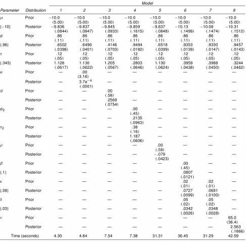
In Table 1 we report means and standard errors (numbers in parentheses) of both prior and posterior distributions, as well as the computing time to generate 100 iterations for each of the eight models. The numbers in square brackets are the true values of the parameters. In Table 2 we report Chib’s marginal
likelihood, harmonic mean, and DIC together with DN andpD
for each of the eight models as well as their associated rank-ings by each criterion. For SV Models 1–5, after a burn-in pe-riod of 50,000 iterations and a follow-up pepe-riod of 250,000, we stored every 20th iteration. Due to higher posterior correla-tions among the parameters and thus slower convergence of the Gibbs sampler in the remaining models, we chose a burn-in pe-riod of 100,000 iterations, a follow-up pepe-riod of 900,000, and stored every 40th iteration. All calculations were performed on a Pentium-III PC, 550 MHz, running the WinBUGS 131 ver-sion updated with the DIC tool.
From the examination of these two tables, we rst note that the correct model (Model 6) is estimated by MCMC with rea-sonably accurate results for all six parameters. Moreover, the
Table 1. Parameter Estimates for Simulated Data
Model
Parameter Distribution 1 2 3 4 5 6 7 8
¹ Prior ¡10:0 ¡10:0 ¡10:0 ¡10:0 ¡10:0 ¡10:0 ¡10:0 ¡10:0
.5:00/ .5:00/ .5:00/ .5:00/ .5:00/ .5:00/ .5:00/ .5:00/
[¡10] Posterior ¡9:836 ¡9:837 ¡9:845 ¡9:859 ¡9:837 ¡10:13 ¡10:08 ¡10:31
.:0844/ .:0847/ .:0933/ .:1615/ .:0848/ .:1499/ .:1474/ .:1512/ Á Prior :86 :86 :86 :86 :86 :86 :86 :86
.:11/ .:11/ .:11/ .:11/ .:11/ .:11/ .:11/ .:11/
[:96] Posterior :6502 :6496 :4146 :9494 :6518 :9353 :9330 :9457
.:0398/ .:0401/ .:0703/ .:0182/ .:0399/ .:0139/ .:0147/ .:0143/ ¿ Prior :12 :12 :12 :12 :12 :12 :12 :12
.:05/ .:05/ .:05/ .:05/ .:05/ .:05/ .:05/ .:05/
[:345] Posterior 1:128 1:130 1:205 :2803 1:130 :3959 :3988 :3244
.:0617/ .:0622/ .:0567/ .:0646/ .:0624/ .:0438/ .:0450/ .:0462/
® Prior — :00 — — — — — —
.3:16/
Posterior — 3:7e¡4 — — — — — —
.:0001/
à Prior — — :00 — — — — —
.:58/
Posterior — — :2569 — — — — —
.:0754/
Á2 Prior — — — :00 — — — —
.:45/
Posterior — — — :2135 — — — —
.:0963/
¿2 Prior — — — :38 — — — —
.:16/
Posterior — — — 1:187 — — — —
.:0606/
½ Prior — — — — :00 — — —
.:58/
Posterior — — — — ¡:079 — — —
.:0423/
¯ Prior — — — — — :00 — —
.:45/
[:1] Posterior — — — — — :0807 — —
.:0121/
· Prior — — — — — :02 :02 —
.:01/ .:01/
[:08] Posterior — — — — — :0727 :0691 —
.:0099/ .:0100/
± Prior — — — — — :05 :05 —
.:02/ .:02/
[:03] Posterior — — — — — :0342 :0348 —
.:0026/ .:0028/
º Prior — — — — — — — 65:0
.36:4/
Posterior — — — — — — — 2:563
.:1866/
Time (seconds) 4:30 4:84 7:54 7:38 31:31 36:45 31:29 42:59
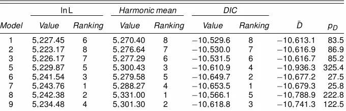
correct model provides the smallest value for DIC as well as for the posterior mean of the deviance despite the fact that the effective number of parameters is not the smallest. We get only
a slightly larger value of DIC for the SVCjumps model
with-out lagged observations (Model 7). This is because differences between this model and the correct model are very small. Not surprisingly, this model is ranked second by DIC. All the other models clearly perform worse. For example, compared with
Table 2. Chib’s Marginal Likelihood, Harmonic Mean, and DIC for Simulated Data
ln L Harmonic mean DIC
Model Value Ranking Value Ranking Value Ranking DN pD
1 6;472:67 7 6;888:43 7 ¡13;442:5 7 ¡14;002:5 560:0 2 6;467:51 8 6;882:43 8 ¡13;441:9 8 ¡14;003:4 561:5 3 6;474:38 5 6;890:43 6 ¡13;463:3 4 ¡14;040:7 577:4 4 6;495:51 4 6;948:43 4 ¡13;496:2 3 ¡14;102:4 606:2 5 6;472:82 6 6;901:42 5 ¡13;453:9 5 ¡14;018:9 565:0 6 6;569:16 1 7;172:00 1 ¡14;450:0 1 ¡14;582:7 132:7 7 6;548:27 2 7;102:92 2 ¡14;362:0 2 ¡14;485:3 123:3 8 6;517:44 3 6;949:62 3 ¡13;448:0 6 ¡14;096:1 648:1
Table 3. Deviance and Harmonic Mean (HM) Summaries for Simulated Data
In fact, the DIC margins among all the models excluding the jump models are reasonably small. For example, DIC of the third best model differs from that of the worst model by 54.3, whereas the difference between the second best and the third best is 865.8. Moreover, the effective number of parameters is much larger for all the models except the jump models and none of these models ts the data as well as the jump models, indi-cated by the highest value for the posterior mean of the
de-viance. Not surprisingly, the higher values ofDN andpDadd up
to the higher DIC values.
Model 4, with two independent AR(1) components, gives a relatively good t, being ranked the best tting after the jump
models by DIC and the best tting after the jump and SV-t
mod-els by Chib’s marginal likelihood. It can thus be considered as a good alternative to using SV models with jumps.
Another interesting result emerging from these two tables is the performance of DIC relative to Chib’s marginal likelihood and the harmonic mean. Neither DIC nor the harmonic mean provides the same model ranking as Chib’s marginal likelihood but the differences are not substantial. Differences between the two marginal likelihood methods and DIC are not surprising as the focus of DIC is different to that of the marginal likelihood methods, as explained in detail in the previous sections.
The computing time to generate 100 iterations suggests that the MCMC program runs substantially slower for the SV Mod-els 5–8 than for the SV ModMod-els 1–4. This is because most of the full conditional distributions for SV Models 5–8 are no longer log-concave and a Metropolis–Hastings updating step is needed. To conserve space, the correlograms are not plotted in the article, but they are available from the authors upon request. Comparison between DIC and Chib’s marginal likelihood
re-veals that the mixture normal-GammatSV model (Model 8) is
the only cause of the discrepancy. Here it is helpful to divide
DIC into a pure measure of tD.µ /N and a measure of
complex-ity 2pDas in (7) to see that thetSV model is heavily penalized
by its high effective number of parameters. ConsideringD.µ /N
gives a value of¡14;715:4 for the true (Model 6) and a value of
¡14;744:1 for thetSV model (Model 8). Thus, thetSV model
provides a better t but its high complexity tips the scales. Al-though not reported, we have also estimated the nonscale
mix-turetSV model and found that the performance of these two
representations are quite different. The nonscale mixturetSV
model performs even worse than the scale mixturetSV model
according to DIC. It has been recognized that different mixture distributions can generate different DIC values, due to the fact
that different mixture distributions correspond to different pre-diction problems, and more research and experience is needed as to the performance of DIC in the area of mixture models (Spiegelhalter et al. 2002).
Table 3 shows the smallest and largest values for DIC and the
harmonic mean, the number of effective parameterspD, and the
goodness of tD, respectively, obtained for six runs for eachN
of the seven models. It serves to demonstrate that DIC varies from one run to another but is reasonably stable across runs. This is in contrast to the well-known instability problem of the harmonic mean, which is apparent from the large discrepancies between the smallest and largest values for the harmonic mean. However, the reader should note that slightly modied estima-tors of the harmonic mean as proposed by Newton and Raftery (1994) are much more stable and do not suffer from the lack of a central limit theorem.
6. AN EMPIRICAL STUDY
6.1 The Data
The dataset consists of 1;512 mean-corrected daily
continu-ously compounded returns,yt, in decimals, on the Standard &
Poors (S&P) 100 index, covering the period of time between January 1993 and December 1998. The S&P 100 index re-turns have been used often in the literature. For instance, Blair, Poon, and Taylor (2001a) estimated the GJR-GARCH model proposed by Glosten, Jagannathan, and Runkle (1993) based on the S&P 100 index returns for four different sample periods from March 1984 to December 1998, one of which is identical to that in this article. We also use data from the Chicago Board Options Exchange Market Volatility Index (VIX) for the same period of time as a covariate, measuring the so-called implied volatility. For a detailed explanation of the Chicago Board Op-tions Exchange Market Volatility Index, the reader is referred to Hol and Koopman (2000) and Fleming, Ostdiek, and Wha-ley (1995). Both data series are plotted in the second and third panels of Figure 1.
6.2 The Models and Prior Distributions
In this section we t the models introduced in Section 5 to the preceding dataset. We drop Model 4 from the list due to a great deal of convergence problems that we have encountered (it may be possible to achieve convergence by using different parameterizations or using different MCMC algorithms, how-ever). Instead we consider as an additional extension a model that includes implied volatility:
Model 9. This model is very similar to the SVX model in-troduced in Hol and Koopman (2000), which includes implied volatility as expressed by an additional covariatext:
ytjhtDexp.ht=2/ut; ut
i:i:d:
» N.0;1/;
htjht¡1; ¹; Á; ¿2; ¸D¹CÁ.ht¡1¡¹/C¸.xt¡ Nx/Cvt;
vt
i:i:d:
» N.0; ¿2/:
The implied volatility is used in this model as an alterna-tive source for predicting volatility and is based on calculations of option price models. The specication of the variance equa-tion is motivated by the empirical result that implied volatilities contain useful information in forecasting future volatilities (see, e.g., Blair, Poon, and Taylor 2001b). In the last panel of Fig-ure 1, we plot the logarithm of the absolute value of S&P 100 returns, which is regarded as an approximation of unobserved log-volatility. It can be seen that the VIX and the logarithm of the absolute value of S&P 100 returns are highly correlated.
Note that we demean the observations in vectorxt for
conver-gence purposes.
A priori,¸is assumed to be uniformly distributed in the
in-terval [¡1;1]. Due to the inclusion of the implied volatility, it is not clear a priori whether the log-volatilityht is still highly
persistent. Instead of using a rather informative prior of a beta distribution with parameters 20 and 1.5 forÁ¤, we choose a less
informative prior forÁ¤, namely, a uniform distribution with
support between 0 and 1.
6.3 Results
In Table 4 we report means and standard errors (numbers in parentheses) of both prior and posterior distributions, as well as the computing time to generate 100 iterations for each of the eight models. For Models 1–5, after a burn-in period of 50,000 iterations and a follow-up period of 250,000, we stored every 20th iteration. In the remaining models, we chose a burn-in pe-riod of 100,000 iterations, a follow-up pepe-riod of 900,000, and stored every 40th iteration.
Table 4. Parameter Estimates for S&P 100 Data
Model
Parameter Distribution 1 2 3 5 6 7 8 9
¹ Prior ¡10:0 ¡10:0 ¡10:0 ¡10:0 ¡10:0 ¡10:0 ¡10:0 ¡10:0
.5:00/ .5:00/ .5:00/ .5:00/ .5:00/ .5:00/ .5:00/ .5:00/
Posterior ¡9:971 ¡9:956 ¡9:986 ¡9:951 ¡10:06 ¡10:07 ¡10:34 ¡9:942
.:2573/ .:2408/ .:2663/ .:2019/ .:2889/ .:2897/ .:3213/ .:0460/ Á Prior :86 :86 :86 :86 :86 :86 :86 :00
.:11/ .:11/ .:11/ .:11/ .:11/ .:11/ .:11/ .:58/
Posterior :9803 :9789 :8375 :9743 :9868 :9873 :9923 ¡:2745
.:0088/ .:0094/ .:1525/ .:0100/ .:0070/ .:0069/ .:0044/ .:1155/ ¿ Prior :12 :12 :12 :12 :12 :12 :12 :12
.:05/ .:05/ .:05/ .:05/ .:05/ .:05/ .:05/ .:05/
Posterior :1674 :1729 :1886 :1947 :1331 :1302 :1005 :4375
.:0297/ .:0317/ .:0442/ .:0319/ .:0284/ .:0286/ .:0189/ .:0763/
® Prior — :00 — — — — — —
.3:16/
Posterior — 1:03e¡4 — — — — — —
.1:7e¡4/
à Prior — — :00 — — — — —
.:58/
Posterior — — :1413 — — — — —
.:1495/
½ Prior — — — :00 — — — —
.:58/
Posterior — — — ¡:4139 — — — —
.:0860/
¯ Prior — — — — :00 — — —
.:45/
Posterior — — — — :0050 — — —
.:0263/
· Prior — — — — :02 :02 — —
.:01/ .:01/
Posterior — — — — :0114 :0115 — —
.:0076/ .:0075/
± Prior — — — — :05 :05 — —
.:02/ .:02/
Posterior — — — — :0315 :0324 — —
.:0119/ .:0121/
º Prior — — — — — — 65:0 —
.36:4/
Posterior — — — — — — 7:306 —
.1:532/
¸ Prior — — — — — — — :0
.:58/
Posterior — — — — — — — :1527
.:0159/
Time (seconds) 3:25 3:66 5:70 23:67 27:56 23:65 32:20 4:27
Table 5. Chib’s Marginal Likelihood, Harmonic Mean, and DIC for S&P 100 Data
ln L Harmonic mean DIC
Model Value Ranking Value Ranking Value Ranking DN pD
1 5;227:45 6 5;270:40 8 ¡10;529:6 8 ¡10;613:1 83:5 2 5;223:17 8 5;276:64 7 ¡10;530:0 7 ¡10;616:9 86:9 3 5;226:17 7 5;277:29 6 ¡10;531:5 6 ¡10;616:7 85:2 5 5;229:87 5 5;300:43 3 ¡10;610:9 4 ¡10;936:3 325:4 6 5;241:54 3 5;279:58 5 ¡10;649:7 2 ¡10;677:2 27:5 7 5;243:76 1 5;288:27 4 ¡10;653:5 1 ¡10;679:3 25:8 8 5;242:38 2 5;331:00 1 ¡10;566:1 5 ¡10;788:9 222:8 9 5;234:48 4 5;301:30 2 ¡10;618:8 3 ¡10;741:3 122:5
From Table 4 it can be seen that the estimated means and standard deviations for the parameters appear quite reasonable and comparable with previous estimates in the literature. For instance, in Model 1, the volatility process is estimated to be
highly persistent. In Model 5 the posterior mean of½is¡:4139
with the upper limit of the 95% posterior credibility interval less than 0. This suggests that the leverage effect is an impor-tant feature for the S&P 100 index. The parameter estimates for
the two SVCjumps models provide similar results for those
parameters already covered by the SV models without jumps. As already observed in Chib et al. (2002), we note that the jump
parameters· and± are not as precisely estimated as other
pa-rameters. However, they are well identied as their posterior distributions are substantially different from their prior
distri-butions. The posterior mean of the jump intensity · is .011,
which means an average daily probability of 1.1% of a jump occurring. This implies that a jump can be expected to occur roughly every 90th day. The standard deviation of the jump size is about .03; that is, daily jumps are usually around 6%.
In Model 8 the posterior mean ofºis 7.306 and similar to the
values of 7.7 and 8.9 for the S&P 500 index in Sandmann and Koopman (1998) and Chib et al. (2002), respectively. The
pos-terior mean of ¸in Model 9 indicates that the implied
volatil-ity contains important information about the volatilvolatil-ity process. Interestingly, allowing for the implied volatility as a covariate induces a negative posterior mean of the autoregressive coef-cient in the model. This nding is similar to what was obtained in Hol and Koopman (2000) based on an S&P 100 index for a different period.
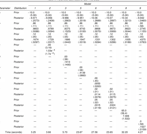
In Table 5 we report Chib’s marginal likelihood, harmonic
mean, and DIC together with DN andpD for each of the eight
models as well as their associated rankings by each criterion. The most adequate models to describe the S&P 100 accord-ing to DIC are the jump model without lagged observations (Model 7) and the jump model with lagged observations (Model 6), followed by the implied volatility model (Model 9)
and the model including the leverage effect (Model 5). Al-though the posterior means of the deviance for the jump models are higher than those of most of the other models, the effective number of parameters is much lower. The effective number of parameters is around 26 for the jump models, which is less than one-third of the effective number of parameters for the clos-est competitor. Model 5 has the lowclos-est posterior means of the deviance, which suggests the best t to the data. However, its effective number of parameters is much higher than that of the other models. In particular, it is more than 10 times larger than that of the jump models. This renders a larger value of DIC.
As for the simulated data, neither DIC nor the harmonic mean provides the same model ranking as Chib’s marginal like-lihood. According to Chib’s marginal likelihood, the strength of evidence to distinguish between the models is much weaker for the S&P 100 data than for the simulated data. For exam-ple, the marginal likelihood values from the second best model and the third best model only differ by .84, which is not worth more than a bare mention according to Jeffrey’s Bayes factor
scale [exp.:84/D2:316]. Nonetheless, both DIC and Chib’s
marginal likelihood select Model 7 (i.e., the jump model with-out lagged observations) as the best performing model, whereas
the harmonic mean picks Model 8 (i.e., thetSV model).
A close look at Table 5 reveals that the mixture
normal-Gamma tSV model (i.e., Model 8) is the major cause of the
discrepancy between the DIC ranking and Chib’s marginal like-lihood ranking. This is a similar nding to the simulated data. Another minor discrepancy arises from the rst three models. Chib’s marginal likelihood ranks Model 2 the worst model, whereas DIC ranks Model 1 the worst.
Table 6 shows the smallest and largest values for DIC and the
harmonic mean, the number of effective parameterspDand the
goodness of tD, respectively, obtained for six runs for each ofN the seven models. Again it demonstrates that DIC varies from one run to another but is reasonably stable across runs and DIC is more stable than the harmonic mean. Also, it can be seen
Table 6. Deviance and Harmonic Mean (HM) Summaries for S&P 100 Data
Model Dmin Dmax pD min pD max DICmin DICmax HMmin HMmax
1 ¡10;617:1 ¡10;611:6 81:9 85:8 ¡10;531:3 ¡10;527:4 5;266:96 5;275:31 2 ¡10;618:4 ¡10;615:9 85:1 88:2 ¡10;531:4 ¡10;529:6 5;271:53 5;279:98 3 ¡10;621:3 ¡10;613:1 83:1 88:8 ¡10;532:8 ¡10;530:0 5;270:33 5;277:29 5 ¡10;941:4 ¡10;934:9 323:0 328:6 ¡10;613:3 ¡10;610:9 5;297:65 5;308:88 6 ¡10;681:5 ¡10;674:9 24:9 29:8 ¡10;656:7 ¡10;645:1 5;279:58 5;287:72 7 ¡10;680:7 ¡10;675:9 24:1 30:3 ¡10;655:1 ¡10;645:7 5;278:56 5;288:27 8 ¡10;791:5 ¡10;787:3 222:2 226:1 ¡10;565:5 ¡10;566:9 5;324:47 5;331:00 9 ¡10;741:5 ¡10;738:8 120:8 124:0 ¡10;618:8 ¡10;617:1 5;298:71 5;302:28
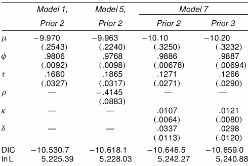
Table 7. Sensitivity of DIC and Chib’s Marginal Likelihood to the Prior
Model 1, Model 5, Model 7
Prior 2 Prior 2 Prior 2 Prior 3
¹ ¡9:970 ¡9:963 ¡10:10 ¡10:20
.:2543/ .:2240/ .:3250/ .:3232/ Á :9806 :9768 :9886 :9887
.:0092/ .:0098/ .:00678/ .:00694/ ¿ :1680 :1865 :1271 :1266
.:0327/ .:0317/ .:0271/ .:0290/
½ — ¡:4145 — —
.:0883/
· — — :0107 :0121
.:0064/ .:0080/
± — — :0337 :0298
.:0113/ .:0120/
DIC ¡10;530:7 ¡10;618:1 ¡10;646:5 ¡10;659:0 ln L 5;225:39 5;228:03 5;242:27 5;240:88
that the ranges of DIC overlap with each other for the rst three models. This explains why the rst three models are difcult to distinguish.
6.4 Robustness Check
In this section we examine the implications of alternative prior distributions on DIC and Chib’s marginal likelihood. In particular, we focus on a subset of hyperparameters, namely,
Áand·. Also, for brevity we only consider a subset of the
mod-els, namely, the basic SV model (Model 1), the SV model with
a leverage effect (Model 5), and the SVCjumps model without
lagged observations (Model 7). Following Chib et al. (2002), we consider the following two alternative priors:
² Prior 2:Á¤»U.0;1/.
² Prior 3:Á¤»U.0;1/; ·»Beta with mean .0385 and stan-dard error .0264.
We reestimate all three models with Prior 2 and Model 7 with Prior 3 and calculate DIC and Chib’s marginal likelihood ac-cordingly. The posterior means, standard errors, DIC, and the marginal likelihood are reported in Table 7. A comparison with the results in Table 4 shows that Prior 2 yields a posterior dis-tribution that is almost identical to that with the original prior and that Prior 3 yields a posterior distribution that is reasonably close to that with the original prior. More important, DIC seems quite robust to the change of prior. Moreover, it preserves the ranking of the models considered and the ranking is consistent with that based on the marginal likelihood.
7. CONCLUSION
In this article we have explored the practical performance of DIC as a model selection criterion for comparing various sto-chastic volatility models. DIC is a Bayesian version of the clas-sical deviance for model assessment. It is particularly suited to compare Bayesian models whose posterior distributions have been obtained using MCMC simulation. Similar to AIC and BIC, DIC comprises two parts, a goodness-of-t measure, the posterior distribution of the deviance, and a penalty term, the ef-fective number of parameters, measuring complexity. Using the
concept ofeffective number of parameters, DIC can be used in
complex hierarchical models where the number of unknowns often exceeds the number of observations and the number of free parameters is not well dened. This is in contrast to AIC and BIC, where the number of free parameters needs to be spec-ied. DIC has been implemented as a tool in the BUGS soft-ware package.
We carry out a simulation study using an SVCjumps model
as the true model. Our estimation results with respect to the simulated data are quite accurate for the true model, and DIC clearly identies the correct model out of eight different
alter-natives. If one were to omit the mixturetSV model, DIC would
give the same model ranking as Chib’s marginal likelihood. By comparing eight different SV models for the S&P 100 index,
comprising 1;512 observations from 1993 to 1998, the jump
volatility model without lagged observations turns out to be the most adequate as indicated by both DIC and Chib’s marginal likelihood. The Monte Carlo error of DIC is fairly low for all the models, indicating a stable performance for model compari-son purposes. Finally, DIC appears robust to the change of prior distributions.
ACKNOWLEDGMENTS
The authors thank an Associate Editor and two anony-mous referees for constructive comments that have substan-tially improved the article. They also acknowledge comments from Nicky Best, Genshiro Kitagawa, Angelika van der Linde, Adrian Pagan, Peter Phillips, Werner Ploberger, and semi-nar participants at the 2001 Australasian Econometric Society Meeting, the New Zealand Econometric Study Group Meeting in Auckland, and the National University of Singapore (both Department of Economics and Center for Financial Engineer-ing). Andreas Berg gratefully acknowledges the support of his research by the DAAD, personal number D/99/19367 within a “DAAD Doktorandenstipendium im Rahmen des gemeinsamen Hochschulsonderprogramms III von Bund und Laendern” and by the Royal Society of New Zealand Marsden Fund for a Ph.D. scholarship under grant 01-UOA-015. The work of Renate Meyer was supported by the Royal Society of New Zealand
Marsden Fund and the University of Auckland Research Com-mittee. Jun Yu acknowledges nancial support from the Univer-sity of Auckland Research Committee and the Royal Society of New Zealand Marsden Fund under grant 01-UOA-015.
[Received October 2001. Revised May 2003.]
REFERENCES
Akaike, H. (1973), “Information Theory and an Extension of the Maximum Likelihood Principle,” inProceedings of the Second International Sympo-sium on Information Theory, eds. B. N. Petrov and F. Csaki, Budapest: Akademiai Kiado, pp. 267–281.
Andersen, T. G., Chung, H.-J., and Sørensen, B. E. (1999), “Efcient Method of Moments Estimation of a Stochastic Volatility Model: A Monte Carlo Study,”
Journal of Econometrics, 91, 61–87.
Andersen, T. G., and Sørensen, B. E. (1996), “GMM Estimation of a Stochastic Volatility Model: A Monte Carlo Study,”Journal of Business & Economic Statistics, 14, 329–352.
Andrews, D. F., and Mallows, C. L. (1974), “Scale Mixtures of Normal Distri-butions,”Journal of the Royal Statistical Society, Ser. B, 36, 99–102. Berger, J. O., and Pericchi, L. R. (1996), “The Intrinsic Bayes Factor for Model
Selection and Prediction,”Journal of the American Statistical Association, 91, 109–122.
Best, N., Cowles, M. K., and Vines, K. (1995), “CODA Convergence Diagnosis and Output Analysis Software for Gibbs Sampling Output Version 0.30,” Cambridge, U.K.: MRC Biostatistics Unit.
Black, F. (1976), “Studies of Stock Market Volatility Changes,”Proceedings of the American Statistical Association,Business and Economic Statistics Section, 177–181.
Blair, B. J., Poon, S.-H., and Taylor, S. J. (2001a), “Modelling S&P 100 Volatil-ity: The Information Content of Stock Returns,”Journal of Banking and Fi-nance, 25, 1665–1679.
(2001b), “Forecasting S&P 100 Volatility: The Incremental Informa-tion Content of Implied Volatilities and High Frequency Returns,”Journal of Econometrics, 105, 5–26.
Bollerslev, T. (1986), “Generalized Autoregressive Conditional Heteroskedas-ticity,”Journal of Econometrics, 31, 307–327.
Brenner, R. J., Harjes, R. H., and Kroner, K. F. (1996), “Another Look at Mod-els of the Short-Term Interest Rate,”Journal of Financial and Quantitative Analysis, 31, 85–107.
Carlin, B. P., and Louis, T. A. (1996),Bayes and Empirical Bayes Methods for Data Analysis,Monographs on Statistics and Applied Probability, 69. Chacko, G., and Viceira, L. M. (2003), “Spectral GMM Estimation of
Continuous-Time Processes,”Journal of Econometrics, 116, 259–292. Chan, K. C., Karolyi, G. A., Longstaff, F. A., and Sanders, A. B. (1992),
“An Empirical Comparison of Alternative Models of the Short-Term Inter-est Rate,”The Journal of Finance, 47, 1209–1227.
Chernov, M., Gallant, A. R., Ghysels, E., and Tauchen, G. (2003), “Alternative Models for Stock Price Dynamics,”Journal of Econometrics, 116, 225–257. Chib, S. (1995), “Marginal Likelihood from the Gibbs Output,”Journal of the
American Statistical Association, 90, 1313–1321.
Chib, S., Nardari, F., and Shephard, N. (1999), “Analysis of High Dimensional Multivariate Stochastic Volatility Models,” unpublished paper.
(2002), “Markov Chain Monte Carlo Methods Stochastic Volatility Models,”Journal of Econometrics, 108, 281–316.
Dempster, A. P. (1974), “The Direct Use of Likelihood for Signicance Test-ing,” inProceedings of Conference on Foundational Questions in Statistical Inference, University of Aarhus, pp. 335–352.
Doucet, A., de Freitas, N., and Gordon, N. (2001),Sequential Monte Carlo Methods in Practice, New York: Springer-Verlag.
Dufe, D., and Singleton, K. J. (1993), “Simulated Moments Estimation of Markov Models of Asset Prices,”Econometrica, 61, 929–952.
Engle, R. F. (1982), “Autoregressive Conditional Heteroscedasticity With Es-timates of the Variance of United Kingdom Ination,”Econometrica, 50, 987–1007.
Engle, R. F., and Ng, V. K. (1993), “Measuring and Testing the Impact of News on Volatility,”The Journal of Finance, 48, 1749–1778.
Fernandez, C., Ley, E., and Steel, M. F. J. (2001), “Benchmark Priors for Bayesian Model Averaging,”Journal of Econometrics, 100, 381–427. Fleming, J., Ostdiek, B., and Whaley, R. E. (1995), “Predicting Stock Market
Volatility: A New Measure,”Journal of Futures Markets, 15, 265–302.
Gallant, A. R., and Tauchen, G. (1996), “Which Moments to Match,” Econo-metric Theory, 12, 657–681.
(2001), “Efcient Method of Moments,” working paper, University of North Carolina, Dept. of Economics. Available at www.unc.edu/arg. Gelman, A., Carlin, J. B., Stern, H. S., and Rubin, D. B. (1996),Bayesian Data
Analysis, London: Chapman & Hall.
George, E. I., and Foster, D. P. (2001), “Calibration and Empirical Bayes Vari-able Selection,”Biometrika, 87, 731–747.
Ghysels, E., Harvey, A. C., and Renault, E. (1996), “Stochastic Volatility,” in
Statistical Models in Finance, eds. C. R. Rao and G. S. Maddala, Amsterdam: North-Holland, pp. 119–191.
Gilks, W. R., Richardson, S., and Spiegelhalter, D. J. (1996),Markov Chain Monte Carlo in Practice, London: Chapman & Hall.
Glosten, L. R., Jagannathan, R., and Runkle, D. E. (1993), “On the Relation Between the Expected Value and the Volatility of the Nominal Excess Return on Stocks,”The Journal of Finance, 48, 1779–1801.
Gordon, N. J., Salmond, D. J., and Smith, A. E. M. (1993), “A Novel Approach to Nonlinear and Non-Gaussian Bayesian State Estimation,”IEEE Proceed-ingsF, 140, 107–133.
Han, C., and Carlin, B. P. (2001), “Markov Chain Monte Carlo Methods for Computing Bayes Factors: A Comparative Review,”Journal of the American Statistical Association, 96, 1122–1132.
Harvey, A. C., Ruiz, E., and Shephard, N. (1994), “Multivariate Stochastic Vari-ance Models,”Review of Economic Studies, 61, 247–264.
Heidelberger, P., and Welch, P. (1983), “Simulation Run Length Control in the Presence of an Initial Transient,”Operations Research, 31, 1109–1144. Hoeting, J. A., Madigan, A., Raftery, A. E., and Volinsky, C. T. (1999),
“Bayesian Model Averaging: A Tutorial,”Statistical Science, 14, 383–417. Hol, E., and Koopman, S. J. (2000), “Forecasting the Variability of Stock Index
Returns With Stochastic Volatility Models and Implied Volatility,” Discus-sion paper, TI 2000-104/4, Tinbergen Institute.
Hull, J., and White, A. (1987), “The Pricing of Options on Asset With Stochas-tic Volatilities,”The Journal of Finance, 42, 281–300.
Jacquier, E., Polson, N. G., and Rossi, P. E. (1994), “Bayesian Analysis of Stochastic Volatility Models” (with discussion),Journal of Business & Eco-nomic Statistics, 12, 371–417.
Kass, R. E., and Raftery, A. E. (1995), “Bayes Factors,”The Journal of the American Statistical Association, 90, 773–795.
Key, J. T., Pericchi, L. R., and Smith, A. F. M. (1999), “Bayesian Model Choice: What and Why?” inBayesian Statistics(Vol. 6), eds. J. M. Bernardo, J. O. Berger, A. P. Dawid, and A. F. M. Smith, Oxford, U.K.: Oxford Univer-sity Press, pp. 343–370.
Kim, S., Shephard, N., and Chib, S. (1998), “Stochastic Volatility: Likelihood Inference Comparison With ARCH Models,”Review of Economic Studies, 65, 361–393.
Kitagawa, G. (1996), “Monte Carlo Filter and Smoother for Gaussian Nonlinear State Space Models,”Journal of Computational and Graphical Statistics, 5, 1–25.
Knight, J. L., Satchell, S. E., and Yu, J. (2002), “Estimation of Stochastic Volatility Model by the Empirical Characteristic Function Method,” Aus-tralian and New Zealand Journal of Statistics, 44, 319–335.
Lavine, M., and Schervish, M. J. (1999), “Bayes Factors: What They Are and What They Are Not,”The American Statistician, 53, 119–122.
Melino, A., and Turnbull, S. M. (1990), “Pricing Foreign Currency Options With Stochastic Volatility,”Journal of Econometrics, 45, 239–265. Meyer, R., and Yu, J. (2000), “BUGS for a Bayesian Analysis of Stochastic
Volatility Models,”The Econometrics Journal, 3, 198–215.
Newton, M. A., and Raftery, A. E. (1994), “Approximate Bayesian Inference With the Weighted Likelihood Bootstrap” (with discussion),Journal of the Royal Statistical Society, Ser. B, 56, 3–48.
O’Hagan, A. (1991), “Contribution to the Discussion of ‘Posterior Bayes Fac-tors,”’Journal of the Royal Statistical Society, Ser. B, 53, 136.
(1994),Kendall’s Advanced Theory of Statistics (Vol. 2), London: Edward Arnold.
Pitt, M., and Shephard, N. (1999a), “Filtering via Simulation: Auxiliary Particle Filter,”Journal of the American Statistical Association, 94, 590–599.
(1999b), “Time Varying Covariances: A Factor Stochastic Volatil-ity Approach” (with discussion), in Bayesian Statistics (Vol. 6), eds. J. M. Bernardo, J. O. Berger, A. P. Dawid, and A. F. M. Smith, Oxford, U.K.: Oxford University Press, pp. 547–570.
Sandmann, G., and Koopman, S. J. (1998), “Estimation of Stochastic Volatility Models via Monte Carlo Maximum Likelihood,”Journal of Econometrics, 87, 271–301.
Schwarz, G. (1978), “Estimating the Dimension of a Model,”Annals of Statis-tics, 6, 461–464.
Shephard, N. (1996), “Statistical Aspects of ARCH and Stochastic Volatil-ity,” inTime Series Models in Econometrics,Finance and Other Fields, eds. D. R. Cox, D. V. Hinkley, and O. E. Barndoff-Nielson, London: Chapman and Hall, pp. 1–67.
Silverman, B. W. (1986),Density Estimation for Statistics and Data Analysis, London: Chapman & Hall.
Singleton, K. J. (2001), “Estimation of Afne Asset Pricing Models Using the Empirical Characteristic Function,”Journal of Econometrics, 102, 111–141. Spiegelhalter, D. J., Best, N. G., Carlin, B. P., and van der Linde, A. (2002), “Bayesian Measures of Model Complexity and Fit” (with discussion), Jour-nal of the Royal Statistical Society, Ser. B, 64, 583–639.
Spiegelhalter, D. J., Thomas, A., Best, N. G., and Gilks, W. R. (1996),BUGS 0.5, Bayesian Inference Using Gibbs Sampling, Manual (Version II), Cam-bridge, U.K.: MRC Biostatistics Unit.
Taylor, S. J. (1982), “Financial Returns Modelled by the Product of Two Sto-chastic Processes—A Study of the Daily Sugar Prices 1961–75,” inTime Se-ries Analysis: Theory and Practice(Vol. 1), ed. O. D. Anderson, Amsterdam: North-Holland, pp. 203–226.
Zhu, L., and Carlin, B. P. (2000), “Comparing Hierarchical Models for Spatio-Temporally Misaligned Data Using the Deviance Information Criterion,”
Statistics in Medicine, 19, 2265–2278.