Full Terms & Conditions of access and use can be found at
http://www.tandfonline.com/action/journalInformation?journalCode=ubes20
Download by: [Universitas Maritim Raja Ali Haji] Date: 11 January 2016, At: 23:08
Journal of Business & Economic Statistics
ISSN: 0735-0015 (Print) 1537-2707 (Online) Journal homepage: http://www.tandfonline.com/loi/ubes20
Forecast Combination Across Estimation Windows
M. Hashem Pesaran & Andreas Pick
To cite this article: M. Hashem Pesaran & Andreas Pick (2011) Forecast Combination Across Estimation Windows, Journal of Business & Economic Statistics, 29:2, 307-318, DOI: 10.1198/ jbes.2010.09018
To link to this article: http://dx.doi.org/10.1198/jbes.2010.09018
Published online: 01 Jan 2012.
Submit your article to this journal
Article views: 292
Forecast Combination Across
Estimation Windows
M. Hashem P
ESARANFaculty of Economics and CIMF, University of Cambridge, Sidgwick Avenue, Cambridge, CB3 9DD, U.K.; and Department of Economics, USC, Kaprielian Hall 300, Los Angeles, CA 90089-0253
Andreas P
ICKEconometric Institute, Erasmus University Rotterdam, Rotterdam 3000 DR, Netherlands; De Nederlandsche Bank;
and CIMF (andreas.pick@cantab.net)
In this article we consider combining forecasts generated from the same model but over different esti-mation windows. We develop theoretical results for random walks with breaks in the drift and volatility and for a linear regression model with a break in the slope parameter. Averaging forecasts over different estimation windows leads to a lower bias and root mean square forecast error (RMSFE) compared with forecasts based on a single estimation window for all but the smallest breaks. An application to weekly returns on 20 equity index futures shows that averaging forecasts over estimation windows leads to a smaller RMSFE than some competing methods.
KEY WORDS: Estimation windows; Exponential down-weighting; Forecast averaging; Structural breaks.
1. INTRODUCTION
There is a sizeable literature on the merits of combining forecasts obtained from different models, reviewed byClemen (1989), Stock and Watson (2004), and, more recently, by Timmermann (2006). Bayesian and equal-weighted forecast combinations are being increasingly used in macroeconomics and finance to good effect. In this literature, the different fore-casts are typically obtained by estimating a number of alterna-tive models over the same sample period.Pesaran and Timmer-mann(2007) argued that the forecast averaging procedure can be extended to deal with other types of model uncertainty, such as the uncertainty over the size of the estimation window, and proposed the idea of averaging forecasts from the same model but computed over different estimation windows. Using Monte Carlo experiments these authors show that this type of forecast averaging reduces the mean squared forecast error (MSFE) in many cases when the underlying economic relations are subject to structural breaks.
The idea of forecast averaging over estimation windows has been fruitfully applied in macroeconomic forecasting. Assenmacher-Wesche and Pesaran (2008) used average fore-casts based on different vector autoregressive models with weakly exogenous regressors (VARX*) of the Swiss economy estimated over different estimation windows and found that averaging forecasts across windows resulted in improvements over averaging of forecasts across models. Similar results were obtained byPesaran, Schuermann, and Smith(2009), who ap-plied the forecast averaging ideas to global VARs composed
of 26 individual country/region VARX* models.Schrimpf and
Wang (2010) applied averaging over estimation windows to
forecasts of GDP growth based on the yield curve. Therefore, it is of interest to see if some theoretical insights can be gained to support these empirical findings.
In this article we derive theoretical results for the average windows (AveW) forecasting procedure. First, we consider a
random walk model. The most interesting case is when the break occurs in the drift term but we also allow for simulta-neous breaks in the drift and volatility of the random walk. We consider single and multiple breaks. We then extend the analy-sis to a linear regression model where the slope coefficient is subject to a break, and show that the results from the random walk model carry over to the linear regression model.
We compare the AveW forecasting procedure with an al-ternative method sometimes used in the literature where the past observations are down-weighted exponentially such that the most recent observations carry the greatest weight in the estimation. Gardner (2006) provided a recent review. We refer to this as the exponential smoothing (ExpS) forecast. In prac-tice, the performance of this approach depends crucially on the choice of the parameter to downweight the past observations.
Initially focusing on a random walk model we show that, in the presence of breaks, the AveW and ExpS forecasting meth-ods always have a lower bias than forecasts from a single esti-mation window. Whereas the MSFE depends on the time and the size of the breaks, the MSFE of the AveW and ExpS fore-casts are smaller than those of the single-window forefore-casts for all but the smallest break sizes.
An attractive feature of these methods is that no exact in-formation about the structural break is needed. This contrasts with the conventional approach of estimating the break points using such methods as those of Bai and Perron (1998,2003), and then basing the forecasts on the post-break observations.
However, as pointed out byPesaran and Timmermann(2007),
it is not always optimal to base forecasts only on the post-break data. Using pre-break data biases the forecast, but also reduces the forecast error variance. The overall effect of using pre-break
© 2011American Statistical Association Journal of Business & Economic Statistics April 2011, Vol. 29, No. 2 DOI:10.1198/jbes.2010.09018
307
data on the MSFE is ambiguous and depends on the size and the point of the break. To optimally exploit information con-cerning parameter breaks in forecasting requires knowing the point and the size of the latest break. Even if the point of the last break can be estimated with some degree of confidence, it is unlikely that the size of the break can be estimated accurately, because it involves estimating the model over the pre-break and post-break periods. If the distance to break (measured from the date on which forecasts are made) is short, then the post-break parameters are likely to be poorly estimated relative to those obtained using pre-break data. In contrast, if the pre-break and post-break samples are both relatively large, then it might be possible to estimate the size of the break reasonably accurately, but in such cases the break information might not be that im-portant. Results from Monte Carlo experiments and from the application to financial time series confirm this intuition.
Closely related to our approach is the suggestion by Clark
and McCracken (2009) that averaging expanding and rolling
windows can be useful for forecasting in the presence of struc-tural breaks. This can be seen as a limited version of AveW forecasts where forecasts from only two different windows are combined.
Another reason for considering the random walk model with drift and volatility instability is that it is generally thought to describe the stochastic properties of many macroeconomic and financial time series. In this article we apply the AveW pro-cedure to forecasting weekly returns on futures contracts for 20 world equity markets. Compared with a range of competing approaches, such as forecasts from rolling windows, expanding windows, ExpS forecasts, and forecasts based on post-break ob-servations with breaks estimated by the sequential procedure of Bai and Perron (1998,2003), the AveW forecast has the lowest RMSFE on average. However, in many cases the differences were not statistically significant, largely reflecting the highly volatile nature of weekly returns.
The rest of the article is organized as follows. Section2sets
out the model, and Section3 develops the AveW forecasting
procedure and establishes its properties. Section4considers the ExpS forecast procedure. Section 5 reports the results of the applications to weekly returns on equity futures, and Section6 concludes. Mathematical details are provided inAppendix A.
2. BASIC MODEL AND NOTATIONS
Consider the following time-varying regression model:
(yt−μy)=βt(xt−μx)+σtεt, εt∼iid(0,1), (1)
which is defined over the sample periodt=1,2, . . . ,T+1 and where the exogenous variable, xt, is assumed to follow a
co-variance stationary process with meanμxand autocovariances,
γx(s), that are absolute summable,∞s=0|γx(s)|<K<∞.
Fur-ther assume that the slope parameter,βt, and the standard
devi-ation,σt, are subject to a break at timet=Tb(1<Tb<T),
βt=
β(1) ∀t≤Tb
β(2) ∀t>Tb,
σt=
σ(1) ∀t≤Tb
σ(2) ∀t>Tb.
The aim is to forecast yT+1 based on the observations
(y1,y2, . . . ,yT) and (x1,x2, . . . ,xT,xT+1). When it is known with certainty that the parameters have not been subject to
breaks, the forecast based on the ordinary least squares (OLS) estimates using all of the available observations is most effi-cient in the mean squared error sense. However, when the para-meters are subject to breaks, more efficient forecasts can be ob-tained. As pointed out earlier,Pesaran and Timmermann(2007) showed that there is typically a trade-off between bias and vari-ance of forecast errors. For example, when there is a break in the slope parameter, the use of the full sample will yield a bi-ased forecast but will continue to have the least variance. On the other hand, a forecast using parameter estimates based on the post-break sample,{yt,xt}Tt=Tb+1,is unbiased but for recent breaks could be inefficient due to a higher variance compared with the full-sample estimate. A third option is to use the
opti-mal window length as suggested byPesaran and Timmermann
(2007). But calculating the optimal window relies on the time and size of the last break. If the break is close to the point of forecast, then reliable estimates of the size of the break cannot be obtained even if the time of the break can be determined accurately. Thus the estimated window length is likely to be suboptimal.
In the absence of reliable information on the point and size of the break(s) inβtandσt, a forecasting procedure that is
reason-ably robust to such breaks will be of interest. In similar fashion to model averaging, which improves forecasts when the opti-mal model is uncertain,Pesaran and Timmermann(2007) con-sidered the use of different sub-windows to forecast and then to average the outcomes, either by using cross-validated weights or simply using equal weights.
Toward this end, consider the sample {yt,xt}Tt=Ti+1, with
0≤Ti<T, which yields an observation window of sizeWi= T −Ti. It is convenient to denote the fraction of
observa-tions in the single window (from the time when the forecast is formed) bywi=(T−Ti)/T. The estimation process could
start with a minimum window,{yt,xt}tT=Tmin+1, of sizewmin= (T−Tmin)/T. Fromwmin, other, larger windows can be consid-ered withTi=Tmin,Tmin−j, . . . ,Tmin−j(m−1), thus yielding mseparate estimation windows withjobservations apart. More specifically, we have
wi=wmin+ i
−1
m−1
(1−wmin) fori=1,2, . . . ,m, (2)
so thatwi∈ [wmin,1]. Clearly,wm=1 corresponds to using the
full sample. The number of estimation windows,m, can be kept fixed asT changes or can be allowed to increase with T. In both cases we must havem≤T(1−wmin)+1. The maximum number of possible windows is set bym=T(1−wmin)+1.For this choice ofm, we have
wi=wmin+ i−1
T , i=1,2, . . . ,T(1−wmin)+1. (3) Similar to the window size, define the distance to the break byb=(T−Tb)/T, withb∈(0,1). The forecast outcomes
de-pend on whetherbis a fixed fraction or changes withT. In the former case,Wb=T−Tb→ ∞asT→ ∞; that is, the number
of post-break observations is large whenTis large. In this case, the point and size of the break can be estimated consistently, as was shown by Bai (1997). Under the latter, we consider the case whereb→0 asT→ ∞,such thatWb=T−Tbis small
even whenT is large. In this case, which is the focus of this
article, the small number of post-break data is likely to lead to imprecise estimates of the point and size of the break.
Given that we consider one-step-ahead forecasts, we assume that no structural breaks occur in the forecast period. (For fore-casting with structural breaks over the forecast period see
Pe-saran, Pettenuzzo and Timmermann2006and Maheu and
Gor-don2008.)
3. AVERAGE WINDOW FORECAST
The AveW forecast is defined by the simple forecast combi-nation rule wi, and forecasts from all windows are given equal weight.
The first object of interest in this article is comparing the single-window forecast, ˆyT+1(w), and the AveW forecasts, ˆ
ym,T+1, in the mean squared error sense. In the case of the
single-window forecast, we focus on the most frequently en-countered case where all observations in a given sample are used. In recursive estimation, the single window can be an ex-panding window or a rolling window, and AveW forecasts can be obtained by averaging over sub-windows within the given expanding or rolling window. Therefore, the AveW procedure is not an alternative to rolling forecasts and can be used irre-spective of whether rolling or expanding windows are used in recursive forecasting.
3.1 Random Walk With Drift
Initially, we focus on a simple version of (1), where μy=
The simplicity of this model allows us to obtain exact finite-sample results for a single break in mean, multiple breaks in mean, and joint breaks in mean and error variance. However, the model is also a forecasting tool for a random walk with drift instability,zt=zt−1+μt+εt, so thatyt=zt, andzˆT+1=
3.1.1 Single Break in Drift and Volatility. In the first in-stance assume that a single break occurs at dateTb, 1<Tb<T,
and suppose that only the mean of the process is subject to the break, namelyμ(1)=μ(2), andσ(1)=σ(2)=σ. In this sim-ple case, the one-step-ahead forecast ofyT+1based on a given
window of sizewT(fromt=T)is given by otherwise. Clearly, if w≤b, then the forecast will have mean μ(2) and will be unbiased. There is, however, a bias when cast error byσ, we have the decomposition
σ−1ξT+1(w)=εT+1+BT+1(w)− which is given and unavoidable; the second term is the “bias” that depends on the size of the break, λ, and the distance to break,b; and the last term represents the estimation uncertainty that depends onTw. The (scaled) MSFE for a window of sizew is given by
MSFE(w)=1+B2T+1(w)+ 1
Tw. (9)
Now consider the forecast from averaging over estimation
windows based on m successive windows of sizes from the
smallest window fractionwminto the largest possible one,wm,
where each forecast is of the form given in (6). The (scaled) one-step-ahead forecast error associated with the average fore-cast is
Thus the bias of the AveW forecast is given by
Bm,T+1=
and, as before, the sign of the bias depends on the sign of (μ(2) −μ(1)). In this case the computation of the vari-ance of the forecast error is complicated due to the cross-correlation of forecasts from different windows. LetνT(wi)=
(1/(Twi))Tt=T(1−wi)+1εt, then Cov[νT(wi), νT(wj)] =
Thus in this case, the scaled MSFE is given by
MSFE(m,wmin;λ,b)=1+B2m,T+1+σ−2Var(yˆm,T+1), (12) withBm,T+1and Var(yˆm,T+1)as defined earlier.
The difference between the scaled MSFE of the single-window forecast (9) and that of the AveW forecast (12) is
This depends on a number of parameters, including the size of the single window,wa. Consider two cases:wa=bandwa>b.
Whenwa=b, the forecast from the single window is unbiased,
whereas the AveW forecast withwm>bis biased. The variance
of the single-window forecast,σ2/(Tb), will be very large when Tbis small, and forecasting from a postbeak sample might not be desirable.
Now assume thatwa>b. In this case we can setwm=wa;
that is, the AveW forecast is constructed from sub-windows within the expanding or rolling window.
Proposition 1. For DGP (5) with givenT andb, the single-window forecast with wa>b has a larger absolute bias than
the AveW forecast with wi, i=1,2, . . . ,T andwm=wa. In
In contrast, the difference between the variance terms is am-biguous. Thus there may be a trade-off between a reduction in the bias and an increase in the variance. Whether or not the AveW forecast has a lower MSFE depends on the length of the single-window forecast,wa, and the minimum window,wmin,
which are chosen by the forecaster, and the break parameters, namely the size and the distance to the break,λandb.
Table 1 illustrates the trade-off numerically. It reports
MSFE(wa;λ,b)−MSFE(m,wmin;λ,b) computed for T = 100, wm =1, and different values of wa, wmin,m, λ, and b.
The top two panels report the results when the single window uses all 100 observations,wa=1. In the lower two panels, the
single window equals the minimum window,wa=wmin. The
first and third panels give the results when the windows in the AveW forecast are one observation apart, the AveW forecasts in the second and fourth panels use 10 equally spaced windows.
First, consider the top two panels. The first line in each panel shows the difference between the MSFE of the single window and that of the AveW window forλ=0, that is, in the absence of a break. In this case, as expected, the single window
outper-forms the AveW forecasts. However, asλ increases, the bias
reduction implied by averaging over estimation windows leads to a decrease in the MSFE of the AveW forecast relative to that of the single-window forecast. The improvement is modest for small breaks, but the difference in MSFEs increases to about a third of the variance of the innovation when the break is equal to the standard deviation of the innovation.
For the range ofbconsidered, the benefit of averaging fore-casts over estimation windows for a givenwminincreases with b, because a larger number of sub-windows over the post-break sample are used. For the same reason, the difference in the MSFEs decreases inwminwhenλ >0. Whenλ=0, a smaller wmin increases the variance of the AveW forecast due to the larger number of correlated forecasts included. The results re-ported in the first line of the first panel form=T(1−min)+1 and those in the first line of the second panel form=10 sug-gest that the variance term of the AveW forecast decreases inm. Whenλincreases, the reduction in the bias leads to a larger re-duction in the MSFE for a smallerm. However, the size of this effect depends onbandwmin. Overall, the numerical examples in the first two panels show that the effects ofb,wmin, andm are of second-order importance compared with the gains from averaging forecasts over estimation windows.
The bottom two panels, which compare the AveW forecast using allT=100 observations and the single window of length wmin, show that for small breaks, the forecast from the short single window has a much larger MSFE than the AveW fore-cast due to the large estimation uncertainty associated with the small single window. Even for largerλ, a single window that is too small leads to an inferior forecast due to the large estima-tion uncertainty. However, whenλis large and the single win-dow is not too small, using only post-break data can improve the forecast. But this procedure still requiresa priori knowl-edge of the break point or its estimation by means of statistical techniques.
To investigate the implications of estimating the break point for the relative performance of the two forecast procedures, we carried out a Monte Carlo experiment that compares the AveW forecast withwmin=0.02 to forecasts obtained from using data after the break date estimated by the sequential procedure pro-posed by Bai and Perron (1998,2003). We searched for up to three break points and used the observations after the last sta-tistically significant break date to generate one-step-ahead fore-casts. We set the trimming parameter to 0.05 and the signifi-cance level to 5%, and allowed for heterogeneous covariance matrices across segments. The results were robust to varying these settings. The data were generated using model (5) with T=100 andσt=1,∀t, for 10,000 replications.
The results in Table2show that the MSFE of the AveW fore-casts is smaller than that of the forefore-casts based on post-break observations whenλ <1, but whenλ=1, the post-break data forecasts have a lower MSFE. This contrasts with the results in the bottom two panels of Table1where the post-break data forecast has a lower MSFE forλ=0.75. The uncertainty of the time of the break leads to deterioration of the forecast precision
Table 1. MSFE(wa;λ,b)−MSFE(m,wmin;λ,b): Exact results for a single break in drift
b: 0.05 0.1 0.2
λ wmin: 0.02 0.05 0.02 0.05 0.1 0.02 0.05 0.1 0.15 0.2
wa=1,m=T(1−wmin)+1
0 −0.009 −0.008 −0.009 −0.008 −0.007 −0.009 −0.008 −0.007 −0.006 −0.005 0.1 −0.007 −0.006 −0.006 −0.005 −0.004 −0.005 −0.004 −0.003 −0.002 −0.002
0.2 0.001 0.000 0.005 0.005 0.004 0.007 0.008 0.008 0.007 0.007
0.4 0.030 0.024 0.047 0.043 0.035 0.056 0.054 0.051 0.047 0.041
0.75 0.127 0.105 0.186 0.170 0.140 0.218 0.210 0.196 0.178 0.156
1 0.233 0.192 0.337 0.309 0.255 0.394 0.380 0.353 0.320 0.281
wa=1,m=10
0 −0.013 −0.009 −0.013 −0.009 −0.007 −0.013 −0.009 −0.007 −0.006 −0.005 0.1 −0.010 −0.007 −0.010 −0.006 −0.004 −0.009 −0.005 −0.003 −0.003 −0.002
0.2 −0.001 0.002 0.002 0.005 0.005 0.003 0.007 0.008 0.008 0.007
0.4 0.034 0.035 0.048 0.046 0.043 0.053 0.054 0.053 0.049 0.045
0.75 0.154 0.148 0.201 0.187 0.167 0.219 0.214 0.204 0.188 0.172
1 0.285 0.269 0.368 0.339 0.303 0.400 0.388 0.369 0.338 0.310
wa=wmin,m=T(1−wmin)+1
0 0.481 0.182 0.481 0.182 0.083 0.481 0.182 0.083 0.051 0.035
0.1 0.475 0.175 0.476 0.177 0.078 0.479 0.180 0.081 0.048 0.032
0.2 0.455 0.154 0.463 0.163 0.062 0.472 0.172 0.072 0.038 0.021
0.4 0.375 0.070 0.407 0.103 −0.004 0.443 0.142 0.039 0.001 −0.022
0.75 0.109 −0.213 0.220 −0.095 −0.225 0.348 0.040 −0.074 −0.126 −0.164
1 −0.180 −0.521 0.017 −0.311 −0.465 0.244 −0.070 −0.197 −0.263 −0.319 wa=wmin,m=10
0 0.477 0.181 0.477 0.181 0.083 0.477 0.181 0.083 0.051 0.035
0.1 0.471 0.174 0.472 0.176 0.078 0.474 0.178 0.080 0.048 0.032
0.2 0.453 0.156 0.460 0.162 0.063 0.468 0.171 0.072 0.039 0.022
0.4 0.380 0.081 0.408 0.107 0.003 0.440 0.142 0.041 0.003 −0.017
0.75 0.137 −0.170 0.236 −0.079 −0.198 0.349 0.044 −0.066 −0.116 −0.148
1 −0.128 −0.443 0.048 −0.281 −0.417 0.250 −0.062 −0.181 −0.245 −0.290
NOTE: This table reports the difference in the exact MSFE of the single-window forecast for a givenwa, and the AveW forecast withwm=1 given in (13), namely MSFE(wa;λ,b)−
MSFE(m,wmin;λ,b), whenT=100 for different numbers of estimation windows,m, break sizes as a proportion of the standard deviation of the disturbance term,λ, distance to break,
b, and different minimum window sizes,wmin.
and favors the AveW forecast, which does not use estimates of the break dates.
Now also consider a break in the error variance. For sim-plicity of exposition, assume that drift and volatility break at the same time. The one-step-ahead forecast error for a win-dow of sizewis given byξT+1(w)=σ(2)εT+1+BT+1(w)−
1
Tw T
t=T(1−w)+1σtεt.The scaled MSFE for the single-window
Table 2. MSFE(wˆa(BP);λ,b)−MSFE(m,wmin;λ,b): Monte Carlo results for a single break in drift
λ\b 0.05 0.1 0.2
0.1 0.156 0.155 0.134
0.2 0.157 0.158 0.140
0.4 0.164 0.162 0.164
0.75 0.123 0.121 0.109
1 −0.040 −0.242 −0.014
NOTE: This table reports the difference between the MSFE of the forecast based on post-break data, where the break date is estimated using the sequential procedure proposed by Bai and Perron (1998,2003), MSFE(wˆa(BP);λ,b), and that of the AveW forecast, namely MSFE(m,wmin;λ,b). The MSFEs are computed using Monte Carlo experiments
with 10,000 replications. Data were generated using DGP (5) withσt=1,∀t,andT=100. The Bai and Perron test procedure was conducted with up to three breaks, trimming of 0.05, and a 5% significance level. Forecasts were then based on observations after the last detected break. The AveW forecast usedwmin=0.02, windows separated by one
observa-tion, andwm=1.
forecast is
MSFE(wa;λ, κ,b)=1+B2T+1(w)+κ
2wa−b Tw2
a
×I(wa−b)+
min(wa,b) Tw2
a
, (15)
where λ=(μ(2) −μ(1))/σ(2) and κ =σ(1)/σ(2). Similarly, for the AveW forecasts overmestimation windows, the scaled MSFE is
MSFE(m,wmin;λ, κ,b)
=1+B2m,T+1
+m12
κ2 m
i=1 wi−b
Twi
I(wi−b)
1 wi +
2
m
j=i+1 1 wj
+
m
i=1
min(wi,b) Twi
1 wi+
2
m
j=i+1 1 wj
. (16)
Table3gives numerical examples of the difference in MSFEs when the DGP contains a break in the mean and the error vari-ance, that is, the difference of (15) and (16). Here we concen-trate on forecasts withwa=1 andm=T(1−wmin)+1. The
Table 3. MSFE(wa;λ, κ,b)−MSFE(m,wmin;λ, κ,b): Exact results for a single break in drift and volatility
NOTE: This table reports the difference in the exact MSFE of the single-window forecast withwa=1 given in (15) and the AveW forecast withwm=1 given in (16), namely MSFE(wa;λ, κ,b)−MSFE(m,wmin;λ, κ,b), whenT=100, andm=T(1−wmin)+1, for different break sizes,λ, in the drift term measured in
terms ofσ(2), break sizes in the error variances,κ, the distance to the break,b, and different minimum window sizes,w
min.
results depend on whether the error variance increases or de-creases after the break. In the former case, the MSFEs are not much affected by the break in volatility. But the outcome is very different when the error variance decreases after the break. When the distance to the break,b, is small, many of the esti-mation windows in the AveW procedure cover periods of high variance, resulting in large MSFEs. However, as b increases, more of the estimation windows in the AveW procedure fall in the low-variance part of the sample, and AveW offers signifi-cant improvements over the single-window forecast.
3.1.2 Multiple Breaks in Drift. Consider a random walk
model where the drift term is subject tondifferent breaks. De-note the break points bybi,i=1,2, . . . ,n, such thatb1>b2> · · ·>bn,and let the means of the process over these segments
beμ(1), μ(2), . . . , μ(n+1).Specifically,
yt=μt+σ εt fort=1,2, . . . ,T, (17)
such that if the sample period is mapped to the unit interval, then the mean fromt=1 tot=b1Tis given byμ(1), the mean fromt=b1T+1 tot=b2T isμ(2), and so forth.
To simplify the analysis, first assume thatn=2 and note that the one-step-ahead forecast of yT+1 based on the window of sizewT (fromt=T) is given by
From the foregoing results, it is clear that for the case ofn breaks, we have forecast bias per break will be
¯
In contrast, the bias of the AveW forecast is
¯
The variance term is unaffected by the possibility of multiple breaks in the mean.
If we further assume that the break points are uniformly dis-tributed over the sample [i.e., bi ∼U(0,1)], then we have solute expected bias of the single-window forecast and that of the AveW forecast is |E[ ¯BT+1(1)]| − |E(B¯m,T+1)| = |¯λ|(1− wmin)/2≥0, which increases in the absolute average break size, |¯λ|, and decreases in the minimum window size, wmin. Equality holds only when|¯λ| =0.
3.2 Break in the Slope Parameter
Now consider the more general model (1) and assume that
a single break occurs in the slope parameter of the process at date,Tb, 1<Tb<T, whereas the error variance is constant,
namelyβ(1)=β(2), andσ(1)=σ(2)=σ. In this case, the con-ditional (onxT+1) one-step-ahead forecast ofyT+1 based on a given window of sizewTis
ˆ
Under the assumption that xt is a covariance stationary
process with meanμxand absolute summable autocovariances,
∞
seeAppendix A. The estimate of the slope coefficient can be written as
where the first term on the right side of (22) can be rewritten as
T
gressors realized over the estimation window. To simplify the analysis, we can replaceθ (x,w,b)by its mean computed with
respect to the assumed distribution of the regressors. When xt ∼iid N(0, σx2), using the results of Pesaran and
Timmer-mann (2007, app. C), we have that E[θ (x,w,b)] =1.
Simu-lations not reported here but available from the authors show
that this is true for a range of distributions forxt. In what
fol-lows, we work withθ (x,w,b)≈1. In this case, it can be seen
from (24) that the bias is proportional to the size of the break, (β(1)−β(2)), and the proportion of pre-break observations in the sample,(w−b)/w.
Lemma 1. Denote the forecast error based on a single fixed estimation window,w∈ [wmin,1],and a given break pointb∈ (0,1),byξT+1(w)=yT+1− ˆyT+1(w),whereyT+1 is defined by the DGP in model (1) andyˆT+1(w)is given by (19). Define λ=(β(2)−β(1))/σ. Then, conditional onxT+1, for fixedwand
b, the (scaled) forecast error is
σ−1ξT+1(w)=εT+1+
Tb).Now consider the forecast based on aver-aging the forecasts over the different windows,w1,w2, . . . ,wm,
to a single break. Consider the forecast error of the AveW fore-casts based onmestimation windows, defined by (26) and (19). Letζ (wi)= [(wi−b)/wi]I(wi−b),andλ=(β(2)−β(1))/σ.
We are now in a position to compare the MSFE of the stan-dard forecasts based on a single window with the AveW fore-casts. First, consider the case wherebis fixed asT→ ∞.
Proposition 2. Consider the DGP given by (1) with a single break inβt. For largeT but a fixedb such thatWb→ ∞,the
MSFE of the forecast from a single window of lengthbwill be unbiased and will have the lowest MSFE.
This follows directly from the arguments of Bai (1997).
Clearly, under such circumstances, averaging over estimation windows will not improve the forecast accuracy.
However, our focus is on the case where Wbremains small
asT→ ∞. In this case, the forecast using only post-break data will still be unbiased, but the terms of orderOp(√1W
b)will be
large whenWb is small, and the variance of the forecast error
might be quite high. As shown by Pesaran and Timmermann (2007), in such circumstances a larger estimation window might be more appropriate. Accordingly, in what follows we compare a single-window forecast with window sizewa>bto the AveW
forecast based onmwindows starting withw1and ending with wm=wa. In this setup, we have
σ−1 ξT+1(1)−ξm,T+1
=λ(xT+1−μx)
ζ (wa)−
1 m
m
i=1 ζ (wi)
+Op
1 √
T
. (29)
Proposition 3. Suppose that the DGP in (1) holds and is sub-ject to a single break inβt atb. For largeTbut a smallWb, the
MSFE of the forecast from a single window of lengthwa>b
will be larger than that of the AveW forecast withwm=waand
a fixed number of windows,m>1.
This follows because the difference in square brackets in (29) is positive, which follows from Proposition1.
4. FORECASTS FROM TIME–VARYING
PARAMETER MODELS
As an alternative to averaging forecasts over estimation win-dows, we consider time-varying parameter models. Recently, Branch and Evans (2006) considered a number of variations on this class of models and showed that a particularly simple form, known as the “constant gain least squares,” works reasonably well in forecasting U.S. inflation and GDP growth.
Constant gain least squares is equivalent to discounting past observations at a geometric rate, γ (Branch and Evans2006, p. 160). To analyze this forecasting method, we return to the simple model (5) with a break in mean. We denote the constant gain least squares or exponential smoothing (ExpS) forecast by
ˆ
yT+1(γ )=
1−γ
1−γT T
j=1
γT−jyj. (30)
Now consider the case where the mean of yt is subject to a
single break at date Tb, 1<Tb<T, with μ(1) =μ(2) and
σ(1)=σ(2)=σ. The bias of the one-step-ahead forecast er-ror is Bias[ˆyT+1(γ )] =(μ(2)−μ(1))(γ
T−Tb+1−γT
1−γT )(Pesaran and
Pick2008). Because 0< γ <1, the sign of the forecast bias is the same as the sign of(μ(2)−μ(1)). The forecast error vari-ance is given by Var[ξT+1(γ )] =σ2[1+(11−−γγT)2(
1−γ2T
1−γ2 )].It is
interesting to note that for all values ofγ∈(0,1), the sampling variance of the forecast error (the second part in square brack-ets) does not vanish even forTsufficiently large. Therefore, the
exponential down-weighting of the past observations can work only through bias reduction.
The scaled one-step-ahead MSFE in then given by
MSFE(γ;λ,b)=1+λ2
γ1+Tb−γT
1−γT 2
+
1
−γ 1−γT
21
−γ2T 1−γ2
, (31)
whereλ= |μ(2)−μ(1)|/σ. It can be shown that for a suffi-ciently largeT, there is a uniqueγ that minimizes the MSFE.
However, choosing the optimal down-weighting parameterγ
will depend onλandb, which typically are unknown.
Table 4 gives a numerical illustration of the difference in the MSFE of the ExpS forecast and that of the AveW fore-cast, where the AveW forecast uses estimation windows one observation apart. The ExpS forecasts are based on two differ-ent choices of the down-weighting parameter, namelyγ=0.95 and 0.99. The results suggest that whereas b and wmin have some influence on the final outcomes, the choice of the down-weighting parameter dominates the results. Whenγ=0.95, the AveW forecast has a lower MSFE for small breaks, whereas the ExpS forecast has a lower MSFE for larger breaks. This com-parison is reversed whenγ=0.99.
To understand these numerical results, we can express the AveW model as a “forgetting factor” model. Forgetting factor models weigh observations{yt}Tt=1 by factors{kT−t}Tt=1
(Han-nan and Deistler1988; Brailsford, Penm, and Terrell2002). The ExpS model fits naturally into this framework. Using (3) and (4), the AveW forecast can be expressed as
ˆ
ym,T+1=
1 T(1−wmin)+1
×
T(1−wmin)+1
i=1
1 Twmin+i−1
T
t=T(1−wmin)−i+2
yt,
where we use the AveW forecast with windows increasing by one observation. Thus each observationyt,t=1,2, . . . ,T,
re-ceives the weight
k(T,t,wmin)=
1 T(1−wmin)+1
×
t
i=1 1
T+1−iI[T(1−wmin)+1−i]. (32)
Table 4. MSFE(γ;λ,b)−MSFE(m,wmin;λ,b): Exact results for a single break in drift
γ=0.95 γ=0.99
b: 0.1 0.2 0.1 0.2
λ wmin: 0.05 0.1 0.05 0.1 0.2 0.05 0.1 0.05 0.1 0.2
0.1 0.006 0.007 0.007 0.008 0.009 −0.005 −0.004 −0.005 −0.004 −0.003 0.2 0.001 0.000 0.003 0.003 0.001 0.001 0.000 0.003 0.003 0.001 0.4 −0.020 −0.027 −0.014 −0.017 −0.028 0.026 0.018 0.031 0.028 0.018 0.75 −0.089 −0.119 −0.070 −0.085 −0.125 0.108 0.078 0.127 0.112 0.072 1 −0.164 −0.219 −0.131 −0.158 −0.230 0.197 0.143 0.231 0.203 0.132
NOTE: This table reports the difference in the exact MSFE of the ExpS forecast given in (31) and the AveW forecast withwm=1 given in (12), namely
MSFE(γ;λ,b)−MSFE(m,wmin;λ,b), whenT=100,m=T(1−wmin)+1, for different break sizes,λ, defined as a proportion of the standard deviation
of the disturbance term, the proportion of post-break data,b, the minimum window sizes,wmin, and the down-weighting parameter,γ.
Figure 1. Weights attached to observations in AveW and ExpS fore-casts forT=100. This figure plots the weights attached to each ob-servation in a sample of sizeT=100. The numbers in brackets are the minimum window,wmin, in the case of the AveW weights and the down-weighting parameter,γ, in the case of the ExpS weights.
Figure1 plots the weights attached to each observation in AveW and ExpS forecasts using the minimum windows and down-weighting parameters used in the foregoing numerical example. We consider two different choices of the minimum windows,wmin=0.1 and 0.2, in constructing the weights for the AveW forecast. The weights implied by the AveW forecasts vary much less than the weights implied by the ExpS forecasts.
When γ =0.99, the observations are weighted more evenly
than the weights of AveW for both minimum windows, but
when γ =0.95, past observations are discounted much more
heavily. This largely explains the results in Table4.
5. APPLICATIONS TO FINANCIAL TIME SERIES
We now consider the application of the AveW forecasting procedure to weekly returns on futures contracts for 20 eq-uity indices. Our sample ends on November 24, 2008, and thus covers the highly volatile episodes associated with the credit crunch. Details of the data are given inAppendix B.
We recursively compute one-week-ahead forecasts using var-ious forecasting methods for the mean model (5). The baseline forecast uses the observations after the last break identified by the sequential procedure of Bai and Perron (1998,2003), desig-nated BP, where we search for up to eight breaks and set the trimming parameter to 0.1 and the significance level to 5%.
Whereas Pesaran and Timmermann (2007) showed that
fore-cast accuracy can be improved by using some pre-break obser-vations, we use only post-break observations because this is the more common procedure followed in practice, and exploiting the bias-variance trade-off requires knowledge of the break size, which would introduce further complications into the compar-ative forecasting exercise.
We compare the BP post-break forecasts with two versions of the AveW forecasts. The first version averages forecasts from sub-windows within a rolling window of 156 weeks (equal to three years) usingwmin=0.1. This yieldsWmin=15. The sec-ond AveW forecast averages forecasts from sub-windows in an
expanding window using the same number of minimum
ob-servations, Wmin=15. We use m=10 windows. The results
are qualitatively similar when a larger number of estimation windows is used. We also included forecasts from expanding and rolling windows in our comparisons. For the rolling
win-dows, we considered a rolling window of size Wa=156 and
a minimum rolling window of size Wmin=15. Also, as it
could be argued that the AveW forecasts are performing bet-ter because they are effectively based on a smaller average
window (compared with Wa), we considered a third
rolling-window forecast based on an (average) effective rolling-window size ofW=85, computed as the integer part ofWa(1/10+2/10+
· · · +10/10)/10. Finally, we computed ExpS forecasts using two down-weighting parameters,γ=0.95 and 0.99.
For each series, we calculate the absolute bias, the RMSFE,
and tests for predictive performance of Diebold and
Mari-ano(1995). More precisely, RMSFE=(1nn
t=1ξt2)1/2,where
ξt =yt+1 − ˆyt+1|t, the one-week-ahead forecast, yˆt+1|t, is
based on the observations up to t, and n is the number
of forecasts. We also report the RMSFE and the relative RMSFE; that is for, say, the AveW(Wmin)forecast, we report RMSFE[AveW(Wmin)]/RMSFE(BP), where BP denotes the forecast from the baseline forecast using the observations af-ter the break date estimated by the Bai and Perron procedure. Values smaller than 1 indicate that the baseline forecast has a larger RMSFE than the AveW forecast. The Diebold–Mariano test statistics for predictive ability are calculated for the loss dif-ferentiallt(A,B)=ξtA2 −ξtB2,whereξtAandξtBare the forecast
errors for two forecast methods,AandB.
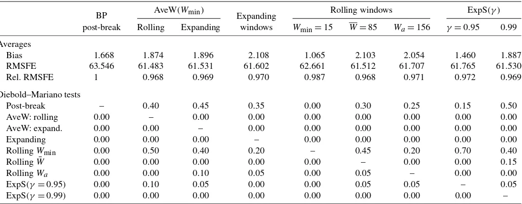
The results are reported in Table5. The first line reports the (absolute) average bias (×100) across the 20 time series, the second line gives the results for the average RMSFE (×100), and the third line presents RMSFE as a ratio of the RMSFE from the forecasts based on the post-break observations. The lower panel of Table 5shows the fraction of series where the test of Diebold and Mariano (1995) rejects equal predictive ac-curacy and the forecast method in the respective column has the lower RMSFE.
The results indicate that the forecasts based on the post-break sample have a smaller average bias than the AveW forecasts but that the average RMSFE is larger than that of the AveW fore-casts. Using DM tests, we find that the AveW forecasts are sta-tistically significantly more accurate in 40% of the series when the AveW forecasts are computed within rolling windows and in 45% of the series if the AveW forecasts are based on expand-ing windows.
Comparing the AveW forecasts with the forecasts based on the corresponding single windows, we find that the AveW fore-casts have a lower bias and RMSFE, as predicted by our the-ory. In contrast, the forecasts from the single rolling window of lengthWminhave a lower bias than the AveW forecasts, because they are less likely to include breaks in the estimation window. However, due to the small number of observations used in the estimation, the RMSFE is larger that that of the AveW fore-casts. The AveW forecasts are significantly more accurate in about half of the series, whereas the short single rolling win-dow is never significantly more accurate than the AveW fore-casts. Comparing the AveW forecasts with the forecasts based
on rolling windows of size W shows that averaging over the
Table 5. Predictive accuracy for alternative forecasts of returns of 20 equity index futures
BP AveW(Wmin) Expanding Rolling windows ExpS(γ)
post-break Rolling Expanding windows Wmin=15 W=85 Wa=156 γ=0.95 0.99
Averages
Bias 1.668 1.874 1.896 2.108 1.065 2.103 2.054 1.460 1.887
RMSFE 63.546 61.483 61.531 61.602 62.661 61.512 61.707 61.765 61.530
Rel. RMSFE 1 0.968 0.969 0.970 0.987 0.968 0.971 0.972 0.969
Diebold–Mariano tests
Post-break – 0.40 0.45 0.35 0.00 0.30 0.25 0.15 0.50
AveW: rolling 0.00 – 0.00 0.00 0.00 0.00 0.00 0.00 0.00
AveW: expand. 0.00 0.00 – 0.00 0.00 0.00 0.00 0.00 0.00
Expanding 0.00 0.00 0.00 – 0.00 0.00 0.00 0.00 0.00
RollingWmin 0.00 0.50 0.40 0.20 – 0.45 0.20 0.70 0.40
RollingW¯ 0.00 0.00 0.00 0.00 0.00 – 0.00 0.00 0.15
RollingWa 0.00 0.00 0.10 0.05 0.00 0.05 – 0.00 0.00
ExpS(γ=0.95) 0.00 0.10 0.05 0.00 0.00 0.05 0.05 – 0.05
ExpS(γ=0.99) 0.00 0.00 0.00 0.00 0.00 0.00 0.00 0.00 –
NOTE: The forecast methods are (i) using the observations after the last break point estimated by the procedure of Bai and Perron (1998,2003); AveW forecasts with the minimum number of observationsWmin=15 weeks andm=10 sub-windows within (ii) a rolling window of lengthWa=156 weeks and (iii) an expanding window; (iv) an expanding window;
single rolling windows of size (v)Wmin=15,(vi)W=85, (vii)Wa=156 weeks; ExpS forecasts with (viii)γ=0.95 and (ix)γ=0.99. The results in the top panel are the absolute
average of the bias across the 20 time series, those in the second row are the average of the RMSFE, and those in the third row are the average of the RMSFE as a ratio of the average RMSFE of the post-break window forecast. The results are multiplied by 100. The lower panel reports the proportion of rejection of predictive accuracy using the test of Diebold and Mariano (1995) across the 20 series. We report the fraction of the series where equal forecast accuracy was rejected and the forecasting method in the respective column had the lower RMSFE than the forecasting method in the respective row. Details of the data are given inAppendix B.
different sub-windows leads to a reduction in bias beyond the implied reduction in sample size. The average RMSFE is re-duced even if this difference is not statistically significant.
The ExpS forecast withγ=0.95, which discounts past ob-servations at a faster rate compared with the ExpS forecasts withγ =0.99, has a lower average bias than the AveW fore-casts and—with the exception of the shortest rolling window— all other forecast procedures. However, the rapid discounting leads to a larger RMSFE than the AveW forecasts and all other forecasting procedures with the exception of the shortest rolling window and the post-break window forecast. The ExpS forecast withγ =0.99 has a smaller average bias than the AveW cast within the expanding window and most of the other fore-cast methods but a larger bias than the AveW forefore-cast within the rolling window. Although the RMSFE is larger than that of the AveW forecasts within the rolling window, it is smaller than that of most other forecast methods.
Overall, it appears that the large variances of the series rel-ative to the size of possible breaks implies that break points are difficult to estimate and forecasts based on such estimates are less precise. Equally, using only short rolling windows in-creases the estimation uncertainty, which eliminates the benefits from the reduction in forecast bias. The same is true of down-weighting observations when the weights decay too rapidly. Us-ing more slowly decayUs-ing weights tends to improve forecast ac-curacy in the MSFE sense. Overall, for the data considered here, the best results are obtained from averaging forecasts over esti-mation windows within a rolling window.
6. CONCLUSION
We have shown that averaging forecasts over estimation win-dows reduces the forecast bias and, despite a potential increase in the variance, reduces the MSFE for all but the smallest
breaks. We have also compared it with the forecast obtained from exponential down-weighting of past observations. Both can be cast in the framework of forgetting factor models. How-ever, the exponential smoothing forecast is more sensitive to the down-weighting parameter than the averaged forecast is to the choice of the minimum estimation window. Monte Carlo results and the application to time series of returns on equity futures show that averaging forecasts over estimation windows can im-prove forecast accuracy compared with forecasts from post-break samples when the variance of the process is relatively large compared with the break size. Averaging of forecasts over different estimation windows offers a simple approach to gener-ating forecasts that are reasonably robust to structural breaks of unknown break dates and sizes. It is likely to be particularly ef-fective when the last break date is relatively close to the point of the forecast and the break is of moderate magnitude. Although our theoretical analysis has been confined to point forecasts for random walk and linear regression models, averaging forecasts over estimation windows is likely to improve forecast accuracy in many settings, such as richer models or density forecasts, but we leave these topics for future research.
APPENDIX A: MATHEMATICAL APPENDIX
Proof of Proposition1
Denoteζ (wi)= [(wi−b)/wi]I(wi−b), and note thatζ (wi)≥
0,∀wi. Furthermore, becauseζ (wi)is increasing inwi,ζ (wa)≥
ζ (wi),∀wi≤wa. Thereforeζ (wa)=m1mi=1ζ (wa)≥(1/m)× m
i=1ζ (wi).Strict equality holds if one element of the last term
contains at least one window for whichwi<wa.
Asymptotic Equivalence ofx¯(w) andμx
Under the assumptions regarding xt in Section 3.2,
limT→∞{Tw[¯x(w)−μx]2} =∞s=−∞γx(s), and for a given w ∈ (wmin,1), wmin > 0, limT→∞{T[¯x(w) − μx]2} =
[∞
s=−∞γx(s)]/w = [2πfx(0)]/w, where fx(0) is the
spec-tral density of{xt}evaluated at zero frequency. Using the
re-sults of propositions 7.5 and 7.11 of Hamilton (1994), then √
Tw), and similarly (becauseεt is serially uncorrelated
with a finite variance) ε(¯ w)=Op(1/√Tw), which yields the
result in (21).
Derivation ofβˆ(w) in (22)
Consider first the denominator ofβ(ˆ w),
1
where the last equality follows from the foregoing argu-ments. Therefore, by Slutsky’s theorem,{Tw1
T
is also exogenously given, and thus given independently ofεt
andxt. Then Var[1/(Tw)TT(1−w)+1(σ εt+βtut)] =σ2/(Tw)+
(24), the forecast error can be written as
ξT+1(w)
With xt being exogeneous, ut and εt are uncorrelated and
(25) follows, noting thatT
t=T(1−w)+1utεt/Tt=T(1−w)+1u2t = Op(1/
√
Tw). Using (A.1), the squared forecast error is
ξT2+1(w)= [σ εT+1+w−wbI(w−b)σ λ(xT+1−μx)]2+Op(1/
The first term does not vary with m. The second term relates to the forecast bias and is bounded inm. Now consider the last
term asT→ ∞, for either a fixedmor asm→ ∞. Using (20),
APPENDIX B: EQUITY INDEX FUTURES AND SAMPLE PERIODS
The equity series refer to futures contracts obtained from Datastream and cover the different periods as set out below. The start of the samples generally coincides with the start dates of the futures markets in question. The last number in the brackets is the number of forecasts.
AEX, Amsterdam exchange index, Netherlands (01-Jun-1989
to 24-Nov-2008; 864);ASX, Australian securities exchange
in-dex (06-Dec-2000 to 19-Nov-2008; 279);BEL, BEL 20 index,
Belgium (07-Jun-1994 to 24-Nov-2008; 603); CAC, CAC 40
index, France (24-Mar-1989 to 24-Nov-2008; 868);DAX, DAX
30 index, Germany (02-Jul-1991 to 24-Nov-2008; 753);DJE,
DJ EURO STOXX 50, DJ euro index (27-Jan-1999 to
25-Nov-2008; 375);FTSE, FTSE 100, U.K. (09-Aug-1985 to
19-Nov-2008; 1054);FOX, FOX index, Finland (02-May-2000 to
19-Nov-2008; 283); IBE, IBEX 35, Spain (25-Nov-1992 to
24-Nov-2008; 672);KFX, KFX index, Denmark (14-Aug-2001 to
25-Nov-2008; 233); MIB, Milan index, Italy (04-Jul-1995 to
20-Nov-2008; 551);ND, NASDAQ 100 index, U.S.A.
(14-Nov-1996 to 21-Nov-2008; 480);NK, NIKKEI 225, Japan
(30-Apr-1987 to 20-Nov-2008; 938); OBX, OBX index, Norway
(26-Aug-1999 to 24-Nov-2008; 326);OMX, OMX index, Sweden
(17-Sep-1990 to 19-Nov-2008; 783);PSI, PSI 20 index, Portu-gal (27-Jan-1997 to 24-Nov-2008; 463);SP, S&P COMP index,
U.S.A. (09-Aug-1985 to 19-Nov-2008; 1050);SMI, SWISS MI
index, Switzerland (18-Jun-1991 to 20-Nov-2008; 766);TPX,
Topix stock price index, Japan (06-Sep-1988 to 19-Nov-2008;
846); TSX, Toronto stock exchange index, Canada
(12-Apr-2000 to 20-Nov-2008; 308).
ACKNOWLEDGMENTS
This article was previously circulated under the title “Fore-casting Random Walks under Drift Instability.” The authors
thank Todd Clark, Jiangqin Fan, (the late) Clive Granger, Alessio Sancetta, Christoph Schleicher, Ron Smith, Vanessa Smith, Jim Stock, two anonymous referees and an associate ed-itor for helpful comments. This article was written while the second author was a Sinopia Research Fellow at the Univer-sity of Cambridge. He acknowledges financial support from Sinopia, quantitative specialist of HSBC Global Asset Manage-ment. The opinions expressed in this article do not necessarily reflect those of De Nederlandsche Bank.
[Received January 2009. Revised February 2010.]
REFERENCES
Assenmacher-Wesche, K., and Pesaran, M. H. (2008), “Forecasting the Swiss Economy Using VECX* Models: An Exercise in Forecast Combination Across Models and Observation Windows,”National Institute Economic Review, 203, 91–108. [307]
Bai, J. (1997), “Estimation of a Change Point in Multiple Regression Models,”
Review of Economics and Statistics, 79, 551–563. [308,313]
Bai, J., and Perron, P. (1998), “Estimating and Testing Linear Models With Multiple Structural Changes,”Econometrica, 66, 47–78. [307,308,310,311,
315,316]
(2003), “Computation and Analysis of Multiple Structural Change Models,”Journal of Applied Econometrics, 18, 1–22. [307,308,310,311,
315,316]
Brailsford, T. J., Penm, J. H. W., and Terrell, R. D. (2002), “Selecting the For-getting Factor in Subset Autoregressive Modelling,”Journal of Time Series Analysis, 23, 629–649. [314]
Branch, W. A., and Evans, G. W. (2006), “A Simple Recursive Forecasting Model,”Economic Letters, 91, 158–166. [314]
Clark, T. E., and McCracken, M. W. (2009), “Improving Forecast Accuracy by Combining Recursive and Rolling Forecasts,”International Economic Review, 50, 363–395. [308]
Clemen, R. T. (1989), “Combining Forecasts: A Review and Annotated Bibli-ography,”International Journal of Forecasting, 5, 559–581. [307] Diebold, F. X., and Mariano, R. S. (1995), “Comparing Predictive Accuracy,”
Journal of Business & Economic Statistics, 13, 253–263. [315,316] Gardner Jr., E. S. (2006), “Exponential Smoothing: The State of the Art—
Part II,”International Journal of Forecasting, 22, 637–666. [307] Hamilton, J. D. (1994),Time Series Analysis, Princeton: Princeton University
Press. [317]
Hannan, E. J., and Deistler, M. (1988),The Statistical Analysis of Linear Mod-els, New York: Wiley. [314]
Maheu, J. M., and Gordon, S. (2008), “Learning, Forecasting and Structural Breaks,”Journal of Applied Econometrics, 23, 553–583. [309]
Pesaran, M. H., and Pick, A. (2008), “Forecasting Random Walks Under Drift Instability,” Working Papers in Economics 0814, University of Cambridge, Faculty of Economics. [314]
Pesaran, M. H., and Timmermann, A. (2007), “Selection of Estimation Window in the Presence of Breaks,”Journal of Econometrics, 137, 134–161. [307,
308,313,315]
Pesaran, M. H., Pettenuzzo, D., and Timmermann, A. (2006), “Forecasting Time Series Subject to Multiple Structural Breaks,”Review of Economic Studies, 73, 1057–1084. [309]
Pesaran, M. H., Schuermann, T., and Smith, L. V. (2009), “Forecasting Eco-nomic and Financial Variables With Global VARs” (with discussion and rejoinder),International Journal of Forecasting, 25, 642–715. [307] Schrimpf, A., and Wang, Q. (2010), “A Reappraisal of the Leading Indicator
Properties of the Yield Curve Under Structural Instability,”International Journal of Forecasting, 26 (4), 836–857. [307]
Stock, J. H., and Watson, M. W. (2004), “Combination Forecasts of Output Growth in a Seven-Country Data Set,”Journal of Forecasting, 23, 405–430. [307]
Timmermann, A. (2006), “Forecast Combinations,” inHandbook of Economic Forecasting,eds. G. Elliot, C. W. J. Granger, and A. Timmermann, Amster-dam: Elsevier, pp. 135–196. [307]