AUTOMATIC RECONSTRUCTION OF BUILDING ROOFS THROUGH EFFECTIVE
INTEGRATION OF LIDAR AND MULTISPECTRAL IMAGERY
Mohammad Awrangjeb, Chunsun Zhang and Clive S. Fraser
Cooperative Research Centre for Spatial Information, Department of Infrastructure Engineering University of Melbourne, Vic 3010, Australia
Phone: +61 3 8344 9182, Fax: +61 3 9654 6515, Email:{mawr, chunsunz, c.fraser}@unimelb.edu.au
Commission III/4
KEY WORDS:Building, Feature, Extraction, Reconstruction, Automation, Integration, LIDAR, Orthoimage
ABSTRACT:
Automatic 3D reconstruction of building roofs from remotely sensed data is important for many applications including city modeling. This paper proposes a new method for automatic 3D roof reconstruction through an effective integration of LIDAR data and multi-spectral imagery. Using the ground height from a DEM, the raw LIDAR points are separated into two groups. The first group contains the ground points that are exploited to constitute a ‘ground mask’. The second group contains the non-ground points that are used to generate initial roof planes. The structural lines are extracted from the grey-scale version of the orthoimage and they are classified into several classes such as ‘ground’, ‘tree’, ‘roof edge’ and ‘roof ridge’ using the ground mask, the NDVI image (Normalised Difference Vegetation Index from the multi-band orthoimage) and the entropy image (from the grey-scale orthoimage). The lines from the later two classes are primarily used to fit initial planes to the neighbouring LIDAR points. Other image lines within the vicinity of an initial plane are selected to fit the boundary of the plane. Once the proper image lines are selected and others are discarded, the final plane is reconstructed using the selected lines. Experimental results show that the proposed method can handle irregular and large registration errors between the LIDAR data and orthoimagery.
1 INTRODUCTION
Up to date 3D building models are important for many GIS appli-cations such as urban planning, and disaster management. Thefore, 3D building reconstruction has been an area of active re-search within the photogrammetric, remote sensing and computer vision communities for the last two decades. Building reconstruc-tion implies the extracreconstruc-tion of 3D building informareconstruc-tion, which in-cludes corners, edges and planes of the building facades and roofs from remotely sensed data such as photogrammetric imagery and height data. Digital reconstruction of the facades and roofs then follows using the available information. Although the problem is well understood and in many cases accurate modelling results are delivered, the major drawback is that the current level of automa-tion is comparatively low (Cheng et al., 2011).
3D building roof reconstruction from aerial imagery seriously lacks in automation partially due to shadows, occlusions and poor contrast. In addition, the extracted information invariably has low vertical accuracy. Fortunately, the introduction of LIDAR has of-fered a favourable option for improving the level of automation in 3D reconstruction when compared to image-based reconstruc-tion alone. However, the quality of the reconstructed building roof from the LIDAR data is restricted by the ground resolution of the LIDAR which is still generally lower than that of the aerial imagery. That is why the integration of aerial imagery and LI-DAR data has been considered complementary in automatic 3D reconstruction of building roofs. However, the question of how to effectively integrate the two data sources with dissimilar char-acteristics still arises; few approaches with technical details have thus far been published.
In the literature, there are two fundamentally different approaches for building roof reconstruction. In themodel drivenapproach, also known as theparametricapproach, a predefined catalogue of roof forms (eg, flat, saddle etc) is prescribed and the model
that fits best with the data is chosen. An advantage of this ap-proach is that the final roof shape is always topologically correct. The disadvantage is, however, that complex roof shapes cannot be reconstructed if they are not in the input catalogue. In addition, the level of detail in the reconstructed building is compromised as the input models usually consist of rectangular footprints. In the
data drivenapproach, also known as thegenericapproach (La-farge et al., 2010), the roof is reconstructed from planar patches derived from segmentation algorithms. The challenge here is to identify neighbouring planar segments and their relations, for ex-ample, coplanar patches, intersection lines or step edges between neighbouring planes. The main advantage of this approach is that polyhedral buildings of arbitrary shape may be reconstructed (Rottensteiner, 2003). However, some roof features such as small dormers and chimneys cannot be represented if the resolution of the input data is low. Moreover, if a roof is assumed to be a com-bination of a set of 2D planar faces, a building with a curved roof structure cannot be reconstructed. Nonetheless, in the presence of high density LIDAR and image data curved surfaces can be well approximated (Dorninger and Pfeifer, 2008). Thestructural
approach, also known as aglobal strategy(Lafarge et al., 2010), exhibits both model and data driven characteristics.
image lines that are parallel or perpendicular to the base line are used to reconstruct the other planes on the same roof. Promising experimental results are provided for both image line classifica-tion and 3D reconstrucclassifica-tion of building roofs.
2 RELATED WORK
The 3D reconstruction of building roofs comprises two important steps (Rottensteiner et al., 2004). Thedetectionstep is a classifi-cation task and delivers regions of interest in the form of 2D lines or positions of the building boundary. Thereconstructionstep constructs the 3D models within the regions of interest using the available information from the sensor data. The detection step significantly reduces the search space for the reconstruction step. In this section, a review of some of the prominent data driven methods for 3D roof reconstruction is presented.
Methods using ground plans (Vosselman and Dijkman, 2001) sim-plify the problem by partitioning the given plan and finding the most appropriate plane segment for each partition. However, in the absence of a ground plan or if it is not up to date, such methods become semi-automatic (Dorninger and Pfeifer, 2008). Rottensteiner (2003) automatically generated 3D building mod-els from point clouds alone. The technique could handle polyhe-dral buildings of arbitrary shape. However, due to use of LIDAR data alone, the level of detail of the reconstructed models and their positional accuracy were poor. In addition, some of the LI-DAR points were left unclassified in the detection step. Later, the detection was improved, along with the reconstruction re-sults, by fusing high resolution aerial imagery with the LIDAR DSM (Rottensteiner et al., 2004), but the objective evaluation re-sults and the assessment of model parameters were still missing. Khoshelham et al. (2005) applied a split-and-merge technique for automatic reconstruction of 3D roof planes. In evaluation, only vertical accuracy of the reconstructed planes from four simple gable roofs was shown. Chen et al. (2006) reconstructed build-ings with straight (flat and gable roofs only) and curvilinear (flat roof only) boundaries from LIDAR and image data. Though the evaluation results were promising, the method could not detect buildings smaller than 30m2
in area and for the detected build-ings both of the planimetric (XY) and shaping (Z) errors were high.
Park et al. (2006) automatically reconstructed large complex buildings using LIDAR data and digital maps. Unlike other meth-ods, the proposed method was able to reconstruct buildings as small as 4m2
; however, in the absence of a ground plan or if it is not up to date, the method is not useful. In addition, objective evaluation results were missing in the published paper. Dorninger and Pfeifer (2008) proposed an automated method using LIDAR point clouds. Since the success of the proposed automated pro-cedure was low, the authors advised manual pre-processing and post-processing steps. In the pre-processing step, a coarse selec-tion of building regions was executed by digitizing each building interactively. In the post-processing step, the erroneous build-ing models were indicated and rectified by means of commercial CAD software. Moreover, some of the algorithmic parameters were set interactively. Sampath and Shan (2010) presented a so-lution framework for segmentation (detection) and reconstruction of polyhedral building roofs from high density LIDAR data. They provided good evaluation results for both segmentation and re-construction. However, due to removal of LIDAR points near the plane boundary the method exhibited high reconstruction errors on small planes. Furthermore, the fuzzy k-means clustering algo-rithm was computationally expensive (Khoshelham et al., 2005). Cheng et al. (2011) integrated multi-view aerial imagery with LI-DAR data for 3D building reconstruction. The proposed method
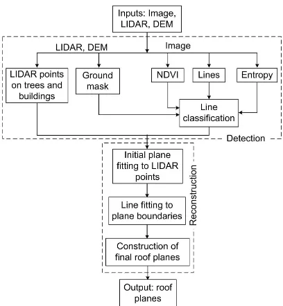
Figure 1: Proposed 3D reconstruction of building roofs.
offered better performance in terms of correctness, completeness and geometric accuracy than a LIDAR-based approach (Sampath and Shan, 2007). However, this was a semi-automatic method since in many cases 20-30% of rooftop lines needed to be manu-ally edited. In addition, this method was computationmanu-ally expen-sive and failed to reconstruct complex roof structures.
3 PROPOSED RECONSTRUCTION PROCEDURE
Figure 1 shows an overview of the proposed building roof re-construction procedure. The input data consist of raw LIDAR data, a DEM and multispectral orthoimagery. The DEM is only used for an estimation of the ground height while generating the mask from the raw LIDAR data. If it is not available, an ap-proximate DEM can be obtained from the input LIDAR data us-ing commercial software, eg the MARS system (MARS Explorer, 2011). In the detection step (top dotted rectangle in Figure 1), the LIDAR points on the buildings and trees are separated as non-ground points. The NDVI (Normalised Difference Vegetation In-dex) is calculated for each image pixel location using the colour orthoimage. The texture information is estimated at each image pixel location using a grey-scale version of the image. The same grey level image is used to find the image lines that are at least 1m in length. These lines are classified into several classes, namely, ‘ground’, ‘tree’, ‘roof edge’ (boundary) and ‘roof ridge’ (inter-section of two roof planes). In the reconstruction step (bottom dotted rectangle in Figure 1), lines classified as roof edges and ridges are processed along with the non-ground LIDAR points. An initial plane fitting uses the LIDAR points near to a long roof edge, which is considered as the base line for the plane. Local image lines are then fit to the boundary points of the plane. The best fitting lines are finally chosen in order to reconstruct a final roof plane. Other planes on the same building are reconstructed following the same procedure by using the non-ground LIDAR points near to the local image lines, which are either parallel or perpendicular to the base line of an already reconstructed plane.
Figure 2: The test scene: (a) orthoimage, (b) LIDAR data shown as a grey-scale grid, (c) NDVI image from (a), and (d) entropy image from (a).
3.1 Test Data Set
Figure 2a presents a test scene which will be used to illustrate the different steps of the proposed reconstruction method. This scene is from Moonee Ponds, Victoria, Australia. Available data comprised of the first-pulse LIDAR data with a point spacing of 1m (Figure 2b), a DEM (with 1m spacing), and an RGBI colour orthoimage with a resolution of 0.1m.
The orthoimage had been created using a bare-earth DEM, so that the roofs and tree-tops were displaced with respect to the LIDAR data. Thus, data alignment was not perfect. Apart from this registration problem, there were also problems with shadows in the orthoimage, so the NDVI image, shown in Figure 2c, did not provide as much information as expected. Therefore, texture information in the form of entropy (Gonzalez et al., 2003) (see Figure 2d) is also employed based on the observation that trees are rich in texture as compared to building roofs. While a high entropy value at an image pixel indicates a texture (tree) pixel, a low entropy value indicates a ‘flat’ (building roof) pixel. The entropy and NDVI information together will be used to classify roof edges and tree edges while classifying image lines.
3.2 Roof Detection
In this section, the LIDAR classification, ground mask generation and image line extraction and classification procedures of the de-tection step in Figure 1 are presented.
3.2.1 LIDAR classification For each LIDAR point, the cor-responding DEM height is used as the ground heightHg. If there is no corresponding DEM height for a given LIDAR point, the av-erage DEM height in the neighbourhood is used asHg. A height thresholdTh=Hg+ 2.5m (Rottensteiner et al., 2004) is applied to the raw LIDAR height. Consequently, the LIDAR data are di-vided into two groups:ground pointswhich reflect from the low height objects such as ground, road furniture, cars and bushes, andnon-ground pointswhich reflect from elevated objects such as buildings and trees.
Figure 3: (a) Ground mask for the scene in Fig 2 and (b) non-ground LIDAR points are overlaid on the orthoimage.
Figure 4: Image lines: (a) extracted and (b) classified (green: ‘tree’, red: ‘ground’, cyan: ‘roof edge’ and blue: ‘roof ridge’).
3.2.2 Mask generation Each of the LIDAR points in the ground point set is marked white in the ground maskMg, which is ini-tially a completely black mask. Therefore, as shown in Figure 3a,Mg indicates thevoid areaswhere there are no laser returns belowTh, i.e., ground areas covered by buildings and trees. This mask will be used to classify image lines into different classes, as described in Section 3.2.4. The non-ground point set (shown in Figure 3b) is preserved for reconstruction of the roof plane, as discussed in Section 3.3.
3.2.3 Image line extraction In order to extract lines from a grey-scale orthoimage, edges are first detected using the Canny edge detector. Corners are then detected on the extracted curves via a fast corner detector (Awrangjeb et al., 2009). On each edge, all the pixels between two corners or a corner and an endpoint, or two endpoints when enough corners are not available, are con-sidered to form a separate line segment. If a line segment is less than 1m in length it is removed. Thus trees having small horizon-tal areas are removed. Finally, a least-squares straight-line fitting technique is applied to properly align each of the remaining line segments. Figure 4a shows the extracted lines from the test scene.
3.2.4 Line classification For classification of the extracted im-age lines, a rectangular area of 1.5m width on each side of a line is considered. The width of the rectangle is based on the assump-tion that the minimum building width is 3m. In each rectangle, the percentageΦof black pixels fromMg(from Figure 3a), the average NDVI valueΥ(from Figure 2c) and the percentageΨ
of pixels having high entropy values (from Figure 2d) are esti-mated. A binary flag Fb for each rectangle is also estimated, whereFb= 1indicates that there are continuous black pixels in
Mg along the line. Note that a pixel having an entropy value of more than 0.8 is considered as a highly textured pixel because this threshold is roughly the intensity value of pixels along the boundary between the textures (Gonzalez et al., 2003).
classi-fied as ‘ground’. Otherwise,ΥandΨare considered for each side whereΦ≥10%. If Υ>10and Ψ>30%(Awrangjeb et al., 2010a) on either of the sides then the line is classified as ‘tree’. If
Υ≤10, or ifΥ>10butΨ≤30%, then the line is classified as ‘roof ridge’ ifFb= 1on both sides. However, ifFb= 1on one side only then it is classified as ‘roof edge’. Otherwise, the line is classified as ‘ground’ (Fb= 0on both sides), for example, for road sides with trees on the nature strip.
3.2.5 Classification performance Figure 4b shows different classes of the extracted image lines. In terms ofcompleteness
andcorrectness(Awrangjeb et al., 2012) the classification perfor-mance was, ‘ground’: 89% and 93%, ‘tree’: 96% and 98%, ‘roof edge’: 87% and 71% and ‘roof ridge’: 95% and 95%. Although ‘tree’ and ‘roof ridge’ classes were identified with high accuracy, there were reasons why ‘ground’ and ‘roof edge’ classes were not always so accurate. Due to shadows (where high NDVI and low entropy were observed) from nearby trees and buildings, some ground lines were classified as roof edges. Due to registration error between LIDAR and image data, many building edges were classified as either roof ridges or ground lines and some building ridges were classified as building edges. Moreover, shadows and registration error, when combined with sudden change in ground height even between neighbouring buildings, resulted in the clas-sification of many ground and tree lines as roof edges and ridges.
Logically, only the lines in classes ‘roof edge’ and ‘roof ridge’ should be considered for reconstruction of roof planes. Since there is some classification inaccuracy in the ‘roof edge’ class, lines classified as ‘roof edge’ or ‘roof ridge’ will be the start-ing edge while reconstructstart-ing a roof plane, but lines in other classes may be considered to complete the plane or to reconstruct a neighbouring plane.
3.3 Roof Reconstruction
In this section, initial plane fitting, image line fitting on the LI-DAR plane boundary and final plane construction procedures of the reconstruction step in Figure 1 are presented.
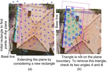
3.3.1 Initial plane fitting The lines in the ‘roof edge’ class are sorted into descending order of their length. Considering the longest roof edge as a base line (see cyan coloured line in Figure 5a) for the corresponding roof plane, a plane is fit to the non-ground LIDAR points as follows.
Ax+By+Cz+D= 0. (1)
Let the LIDAR point spacing be denoted asdf, which is 1m for the test data set. There are 4 unknowns in (1), so at least four LI-DAR points on the actual plane are needed. In order to find these points, a rectangle (width df on each side, magenta coloured solid rectangle in Figure 5a) around the base line is considered. If the required number of points are not found within this rect-angle then the rectrect-angle is extended iteratively, bydf
2 each time, towards the centre of the building. The points which reflect from the wall are not considered. The number of such points is small and their height is low as compared to the actual points on the roof. A point within the rectangle is considered to be reflected from the wall if it has high height difference (more thandf) with majority of the points within the rectangle. Once the required number of points on the plane is obtained, the initial plane using Eq. (1) is constructed.
In order to find whether the roof plane is flat or has an upward or downward slope with respect to the base line, the nearest and the farthest points (PnandPf) from the base line are found. If
PnandPf have similar height, the plane is flat. If the height at
Figure 5: (a) Fitting a plane to the LIDAR points and (b) finding the boundary points of the plane.
Pnis smaller than that atPfthen the plane has an upward slope. Otherwise, it has a downward slope with respect to the base line.
The best-fitting plane is then iteratively extended towards the build-ing centre by considerbuild-ing a rectangle of widthdfoutside the pre-vious rectangle (see magenta coloured dotted rectangle in Figure 5a). As long as at least 1 point within the new rectangle is com-patible (slope and residue of the plane do not change much), the plane is extended. At each iterationPnandPf are updated in order to avoid extending the plane on to a neighbouring plane. The points reflected from the wall are also excluded. Similarly, the plane is extended towards the left and right of the base line as long as the residual of the plane does not increase. Figure 5b shows the fitted plane as a solid magenta coloured rectangle. The points reflected from the wall are shown in red circles and those reflected from the roof plane are shown in either blue coloured squares (boundary of the initial roof plane) or green coloured cir-cles (inside the initial plane boundary).
In order to obtain the boundary points of the plane, the Delaunay triangulation among the fitted points (see cyan coloured triangles in Figure 5b) is constructed. A triangle side that connects the two neighbouring points and constitutes only one triangle should be on the boundary of the plane. However, a triangle side that con-nects two non-neighbouring points but constitutes only one trian-gle is not on the boundary of the plane. To remove such a triantrian-gle side the two inside anglesAandBare checked, as shown in Fig-ure 5b. If any of the angles is less than40◦(ideally,45◦), then
the side of the triangle is removed. As a result, two other sides of that triangle become candidates to be on the boundary of the plane. The corresponding two triangles are then checked to verify their candidacy. This procedure continues until all the outside tri-angles in the triangulation have tri-angles near45◦. This constraint
ensures that the outside triangles connect the neighbouring points only and their sides, each of which constitutes only one triangle, provide the boundary points of the plane.
3.3.2 Image line fitting Since there is registration error be-tween the LIDAR points and orthoimage, the initial plane fitted with the LIDAR points in the previous section may not directly correspond to the image lines on the actual roof plane. Therefore, the solid magenta coloured rectangle in Figure 5b is extended by
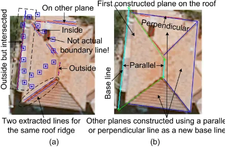
Figure 6: (a) Fitting image lines to an initial plane and (b) con-structed final planes.
Figure 7: Fitting LIDAR plane boundary to an image. The line is: (a) completely inside or outside of the boundary and (b) inter-sected with the boundary.
Due to quantization errors, the extracted image lines may not be aligned properly with respect to the base line. Furthermore, two lines for the same roof ridge may be extracted as shown in the dot-ted ellipse in Figure 6a. The lines which are parallel (within±π
8) or perpendicular (within±π
2 ± π
8) to the base line are obtained and adjusted (Awrangjeb et al., 2010b). In addition, if there are two parallel lines found for the same image line (within a neigh-bourhood of 5 image pixels) then an average line for these two is obtained. Figure 6a shows the adjusted and average lines in red colour.
Because of irregular registration error, each of the image lines obtained as above may be inside, outside or intersected with the boundary points (see Figure 6a). The following rules to catego-rize these image lines are set. For an image line, the boundary points are divided into two groups:insideandoutside. Now with respect to plane boundary the line is:
• completely outside: All the points will be in theinsidegroup, but no points in theoutsidegroup.
• completely inside: There will be no points in theinside
group withindf
2 distance of the line, but in theoutsidegroup there will be at least two points withindf distance of the line.
• outside but intersected: There will only be a few points in theoutsidegroup and they mainly reside withindf
2 distance of the line. However, the majority of the boundary points fall into theinsidegroup and many of them stay withindf distance of the line.
• inside but intersected: In theoutside group there will be only a few points within df
2 distance of the line. But in the
insidegroup there are many points withindfdistance of the line.
The first two cases are illustrated by Figure 7a and the other two by Figure 7b. In fact, some of the lines may not be on the actual plane boundary or may be on neighbouring planes, as shown in Figure 6a. Such lines can be avoided when the number of actual fitted boundary points is counted and only those lines which have high number of fitted points are selected. The fitted points can be easily obtained within the buffer, as shown in Figure 7. For a line which is completely outside or inside of the initial plane boundary, the buffer is situated on the side of the line where the corresponding boundary segment lies, and its width isdm+df, wheredmis the perpendicular distance from the nearest LIDAR boundary point to the base line (see Figure 7a). For an intersected line, the buffer is situated on both sides of the line and its width is1.5df. As shown in Figure 7b, two-thirds of the buffer is situ-ated on the side of the line where the majority of the intersected boundary segment lie.
If there are no or only one fitted point within the defined buffer of a line, then the line is removed. The line which is shown on a neighbouring plane in Figure 6a is thus removed. For each fitted line, the two end LIDAR points from the fitted boundary segment are found.
3.3.3 Final plane construction The image lines with the fit-ted boundary points are now available. The lines which are paral-lel to the base line and have at least two fitted points are the first selected lines (shown in cyan colour in Figure 6b) on the final plane boundary.
Then, the remaining lines (shown in green and red colours in Fig-ure 6b) are sorted into descending order of the number of fitted points. The line which has the maximum number of fitted points is selected and the intersections (shown in green cross signs in Figure 6b) with the already selected lines are found. The ends of the selected lines with new end (intersected) points are recorded. The procedure continues for the rest of the sorted lines. If an end gets two intersection points the earliest one is retained and the new one is discarded. If both of the intersected points of a newly selected line are discarded, the line is also discarded. In Figure 6b, the selected lines are shown in green and discarded lines are in red.
Due to an image line being missed, there may be ends which do not get any intersected points. In such cases, a straight line (using the least-squares technique) is fitted to the LIDAR bound-ary points that reside between the two ends. This straight line is added as a selected line and the intersection points are assigned to the previously unassigned ends. Later when the neighbouring plane is constructed, this line is replaced with the intersected line of the two planes.
In order to assign height to an intersection point, the two corre-sponding LIDAR end points (of the intersecting lines) are checked. If they are the same point, then its height is assigned to the inter-section point. If they are different then the two corresponding lines are checked. If both of them were considered as outside (completely outsideoroutside but intersected) lines in the pro-cess discussed in Section 3.3.2, the height of the nearest LIDAR end point is assigned. Otherwise, the height of the farthest LI-DAR end point is assigned.
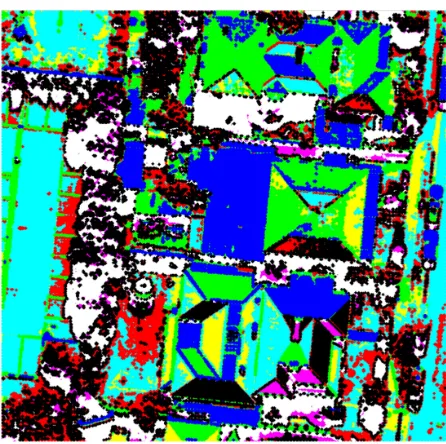
Figure 8: Colour segmentation of the image in Figure 2a.
of a building are reconstructed first before the reconstruction of planes of another building.
4 CONCLUSION AND FUTURE WORK
This paper has proposed a new method for automatic roof recon-struction by integrating LIDAR data and photogrammetric im-agery. In the detection step, image lines are classified into dif-ferent classes. In the reconstruction step, lines in ‘roof edge’ and ‘roof ridge’ classes are primarily employed to fit the LIDAR plane boundaries. Experimental results (Section 3.2.5) show that the detection step can classify the image lines with high accuracy. However, due to shadows, registration error and sudden ground height changes, lines in the ‘ground’ class may also be used. Vi-sual results (Figures 4 to 6) show that the proposed method is capable of handling large and irregular registration error between the two data sources.
The research is ongoing and a comprehensive experimental vali-dation as well as an objective evaluation on different data sets will be essential to proving the effectiveness of the proposed method. In addition, when the density of LIDAR points is low, there may not be a sufficient number of LIDAR points on a small roof ment to construct an initial plane. In such a case, colour seg-mentation of the image can be used to reconstruct the missing planes. Figure 8 shows colour segmentation results using the k-means clustering algorithm. It can be seen that the segmentation results are quite good and small planes can be distinguished from neighbouring planes. Future research will include all the above issues, along with an improvement of the proposed reconstruction method.
ACKNOWLEDGMENT
The authors would like to thank the Department of Sustainability and Environment (www.dse.vic.gov.au) for providing the LIDAR data and orthoimagery for the Moonee Ponds test site.
REFERENCES
Awrangjeb, M., Lu, G., Fraser, C. S. and Ravanbakhsh, M., 2009. A fast corner detector based on the chord-to-point distance accu-mulation technique. In: Proc. Digital Image Computing: Tech-niques and Applications, Melbourne, Australia, pp. 519–525.
Awrangjeb, M., Ravanbakhsh, M. and Fraser, C. S., 2010a. Au-tomatic building detection using lidar data and multispectral im-agery. In: Proc. Digital Image Computing: Techniques and Ap-plications, Sydney, Australia, pp. 45–51.
Awrangjeb, M., Ravanbakhsh, M. and Fraser, C. S., 2010b. Auto-matic detection of residential buildings using lidar data and multi-spectral imagery. ISPRS Journal of Photogrammetry and Remote Sensing 65(5), pp. 457–467.
Awrangjeb, M., Zhang, C. and Fraser, C. S., 2012. Building de-tection in complex scenes thorough effective separation of build-ings from trees. Photogrammetric Engineering and Remote Sens-ing 78(7).
Chen, L., Teo, T., Hsieh, C. and Rau, J., 2006. Reconstruction of building models with curvilinear boundaries from laser scanner and aerial imagery. Lecture Notes in Computer Science 4319, pp. 24–33.
Cheng, L., Gong, J., Li, M. and Liu, Y., 2011. 3d building model reconstruction from multi-view aerial imagery and lidar data. Photogrammetric Engineering and Remote Sensing 77(2), pp. 125–139.
Dorninger, P. and Pfeifer, N., 2008. A comprehensive automated 3d approach for building extraction, reconstruction, and regular-ization from airborne laser scanning point clouds. Sensors 8(11), pp. 7323–7343.
Gonzalez, R. C., Woods, R. E. and Eddins, S. L., 2003. Digital Image Processing Using MATLAB. Prentice Hall, New Jersey.
Khoshelham, K., Li, Z. and King, B., 2005. A split-and-merge technique for automated reconstruction of roof planes. Pho-togrammetric Engineering and Remote Sensing 71(7), pp. 855– 862.
Lafarge, F., Descombes, X., Zerubia, J. and Pierrot-Deseilligny, M., 2010. Structural approach for building reconstruction from a single dsm. IEEE Transactions on Pattern Analysis and Machine Intelligence 32(1), pp. 135–147.
Merrick & Company, 2011. MARS Explorer, Aurora, CO, USA. Version 7.0.
Park, J., Lee, I. Y., Choi, Y. and Lee, Y. J., 2006. Automatic extraction of large complex buildings using lidar data and digital maps. International Archives of the Photogrammetry and Remote Sensing XXXVI(3/W4), pp. 148–154.
Rottensteiner, F., 2003. Automatic generation of high-quality building models from lidar data. Computer Graphics and Ap-plications 23(6), pp. 42–50.
Rottensteiner, F., Trinder, J., Clode, S. and Kubik, K., 2004. Fus-ing airborne laser scanner data and aerial imagery for the auto-matic extraction of buildings in densely built-up areas. In: Proc. ISPRS Twentieth Annual Congress, Istanbul, Turkey, pp. 512– 517.
Sampath, A. and Shan, J., 2007. Building boundary tracing and regularization from airborne lidar point clouds. Photogrammetric Engineering and Remote Sensing 73(7), pp. 805–812.
Sampath, A. and Shan, J., 2010. Segmentation and reconstruc-tion of polyhedral building roofs from aerial lidar point clouds. IEEE Transactions on Geoscience and Remote Sensing 48(3), pp. 1554–1567.