www.elsevier.com/locate/spa
Strong approximation of fractional Brownian motion by
moving averages of simple random walks
Tamas Szabados
Department of Mathematics, Technical University of Budapest, Egry u 20-22, H ep. V em., Budapest, 1521, Hungary
Received 19 December 1999; received in revised form 29 August 2000; accepted 4 September 2000
Dedicated to Pal Revesz on the occasion of his 65th birthday
Abstract
The fractional Brownian motion is a generalization of ordinary Brownian motion, used partic-ularly when long-range dependence is required. Its explicit introduction is due to Mandelbrot and van Ness (SIAM Rev. 10 (1968) 422) as a self-similar Gaussian processW(H)(t) with sta-tionary increments. Here self-similarity means that (a−HW(H)(at):t¿0)=(d W(H)(t):t¿0), where H∈(0;1) is the Hurst parameter of fractional Brownian motion. F.B. Knight gave a construction of ordinary Brownian motion as a limit of simple random walks in 1961. Later his method was simplied by Revesz (Random Walk in Random and Non-Random Environments, World Sci-entic, Singapore, 1990) and then by Szabados (Studia Sci. Math. Hung. 31 (1996) 249 –297). This approach is quite natural and elementary, and as such, can be extended to more general situations. Based on this, here we use moving averages of a suitable nested sequence of simple random walks that almost surely uniformly converge to fractional Brownian motion on compacts whenH∈(1
4;1). The rate of convergence proved in this case is O(N
−min(H−1=4;1=4)logN), where N is the number of steps used for the approximation. If the more accurate (but also more in-tricate) Komlos et al. (1975;1976) approximation is used instead to embed random walks into ordinary Brownian motion, then the same type of moving averages almost surely uniformly con-verge to fractional Brownian motion on compacts for anyH∈(0;1). Moreover, the convergence rate is conjectured to be the best possible O(N−HlogN), though only O(N−min(H;1=2)logN) is proved here. c 2001 Elsevier Science B.V. All rights reserved.
MSC:primary 60G18; 60F15; secondary 60J65
Keywords:Fractional Brownian motion; Pathwise construction; Strong approximation; Random
walk; Moving average
1. Fractional Brownian motion
The fractional Brownian motion (fBM) is a generalization of ordinary Brownian motion (BM) used particularly when long-range dependence is essential. Though the
E-mail address:[email protected] (T. Szabados).
history of fBM can be traced back to Kolmogorov (1940) and others, its explicit in-troduction is due to Mandelbrot and van Ness (1968). Their intention was to dene aself-similar, centered Gaussian process W(H)(t) (t¿0) with stationary but not inde-pendent increments and with continuous sample paths a.s. Here self-similarity means that for any a¿0,
(a−HW(H)(at):t¿0)= (d W(H)(t):t¿0); (1)
whereH∈(0;1) is the Hurst parameterof the fBM and = denotes equality in distri-d bution. They showed that these properties characterize fBM. The case H=12 reduces to ordinary BM with independent increments, while the cases H ¡1
2 (resp. H ¿ 1 2) give negatively (resp. positively) correlated increments; see Mandelbrot and van Ness (1968). It seems that in the applications of fBM, the caseH ¿12 is the most frequently used.
Mandelbrot and van Ness (1968) gave the following explicit representation of fBM as a moving average of ordinary, but two-sided BM W(s); s∈R:
W(H)(t) = 1 (H+12)
Z t
−∞
[(t−s)H−1=2−(−s)H+−1=2] dW(s); (2)
wheret¿0 and (x)+= max(x;0). The idea of (2) is related todeterministic fractional
calculus, which has an even longer history than fBM, going back to Liouville, Riemann, and others; see in Samko et al. (1993). Its simplest case is when a continuous function f and a positive integer are given. Then an induction with integration by parts can show that
f(t) =
1 ()
Z t
0
(t−s)−1f(s) ds
is the order iterated antiderivative (or order integral) off. On the other hand, this integral is well-dened for non-integer positive values of as well, in which case it can be called a fractional integral of f.
So, heuristically, the main part of (2),
W(t) =
1 ()
Z t
0
(t−s)−1W′(s) ds= 1 ()
Z t
0
(t−s)−1dW(s)
is the orderintegral of the (in ordinary sense non-existing) white noise processW′ (t). Thus the fBMW(H)(t) can be considered as a stationary-increment modication of the fractional integralW(t) of the white noise process, where =H+12∈(12;32).
2. Random walk construction of ordinary Brownian motion
enough to hear this version of the construction directly from Pal Revesz in a seminar at the Technical University of Budapest a couple of years before the publication of Revesz’s book in 1990 and got immediately fascinated by it. The result of an eort to further simplify it appeared in Szabados (1996). From now on, the expressionRW constructionwill always refer to the version discussed in the latter. It is asymptotically equivalent to applying Skorohod (1965) embedding to nd a nested dyadic sequence of RWs in BM, see Theorem 4 in Szabados (1996). As such, it has some advantages and disadvantages compared to the celebrated best possible approximation by BM of partial sums of random variables with moment generator function nite around the origin. The latter was obtained by Komlos et al. (1975, 1976), and will be abbrevi-atedKMT approximation in the sequel. The main advantages of the RW construction are that it is elementary, explicit, uses only past values to construct new ones, easy to implement in practice, and very suitable for approximating stochastic integrals, see Theorem 6 in Szabados (1996) and also Szabados (1990). Recall that the KMT ap-proximation constructs partial sums (e.g. a simple symmetric RW) from BM itself (or from an i.i.d. sequence of standard normal random variables) by an intricate sequence of conditional quantile transformations. To construct any new value it uses to whole sequence (past and future values as well). On the other hand, the major weakness of the RW construction is that it gives a rate of convergence O(N−1=4logN), while the rate of the KMT approximation is the best possible O(N−1=2logN), where N is the number of steps (terms) considered in the RW.
In the sequel rst the main properties of the above-mentioned RW construction are summarized. Then this RW construction is used to dene an approximation similar to (2) of fBM by moving averages of the RW. The convergence and the error of this approximation are discussed next. As a consequence of the relatively weaker approxi-mation properties of the RW construction, the convergence to fBM will be established only for H∈(14;1), and the rate of convergence will not be the best possible either. To compensate for this, at the end of the paper we discuss the convergence and error properties of a similar construction of fBM that uses the KMT approximation instead, which converges for all H∈(0;1) and whose convergence rate can be conjectured to be the best possible when approximating fBM by moving averages of RWs.
The RW construction of BM summarized here is taken from Szabados (1996). We start with an innite matrix of i.i.d. random variablesXm(k),
P{Xm(k) = 1}=P{Xm(k) =−1}=12 (m¿0; k¿1);
dened on the same underlying probability space (;A;P). Each row of this matrix
is a basis of an approximation of BM with a certain dyadic step size t= 2−2m in
time and a corresponding step size x= 2−m in space, illustrated by the next table.
The second step of the construction istwisting. From the independent random walks (i.e. from the rows of Table 1), we want to create dependent ones so that after shrinking temporal and spatial step sizes, each consecutive RW becomes a renement of the previous one. Since the spatial unit will be halved at each consecutive row, we dene stopping times byTm(0) = 0, and fork¿0,
Table 1
The starting setting for the RW construction of BM
t x i.i.d. sequence RW
1 1 X0(1); X0(2); X0(3); : : : S0(n) =Pn k=1X0(k) 2−2 2−1 X1(1); X1(2); X1(3); : : : S1(n) =Pn
k=1X1(k)
2−4 2−2 X
2(1); X2(2); X2(3); : : : S2(n) =P
n k=1X2(k) .
.
. ... ... ...
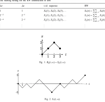
Fig. 1.B0(t;!) =S0(t;!).
Fig. 2.S1(t;!).
These are the random time instants when a RW visits even integers, dierent from the previous one. After shrinking the spatial unit by half, a suitable modication of this RW will visit the same integers in the same order as the previous RW. (This is what we call a renement.) We will operate here on each point !∈ of the sample space separately, i.e. we x a sample path of each RW appearing in Table 1. Thus each
bridgeSm(Tm(k+ 1))−Sm(Tm(k)) has to mimic the corresponding step Xm−1(k+ 1) of the previous RW. We dene twisted RWs ˜Smrecursively for m= 1;2;3; : : :using ˜Sm−1, starting with ˜S0(n) =S0(n) (n¿0). With each xed m we proceed for k= 0;1;2; : : : successively, and for every n in the corresponding bridge, Tm(k)¡n6Tm(k+ 1). Any
bridge is ipped if its sign diers from the desired (Figs. 1–3):
˜ Xm(n) =
(
Xm(n) if Sm(Tm(k+ 1))−Sm(Tm(k)) = 2 ˜Xm−1(k+ 1);
−Xm(n) otherwise;
and then ˜Sm(n) = ˜Sm(n −1) + ˜Xm(n). Then each ˜Sm(n) (n¿0) is still a simple,
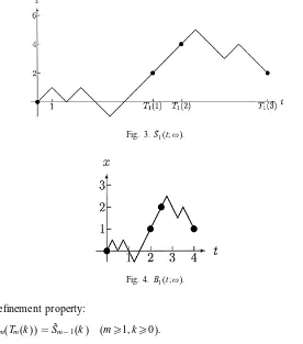
Fig. 3. ˜S1(t;!).
Fig. 4.B1(t;!).
desired renement property:
1
2S˜m(Tm(k)) = ˜Sm−1(k) (m¿1; k¿0): (3)
The last step of the RW construction is shrinking. The sample paths of ˜Sm(n) (n¿0)
can be extended to continuous functions by linear interpolation. This way one gets ˜
Sm(t) (t¿0) for realt. Then we dene themth approximation of BM (see Fig. 4) by
Bm(t) = 2−mS˜m(t22m): (4)
Compare three steps of a sample path of the rst approximation B0(t;!) and the corresponding part of the second approximationB1(t;!) on Figs. 1 and 4. The second visits the same integers (dierent from the previous one) in the same order as the rst, so mimics the rst, but the corresponding time instants dier in general: 2−2T
1(k)6=k. Similarly, (3) implies the generalrenement property
Bm+1(Tm+1(k)2−2(m+1)) =Bm(k2
−2m) (m¿0; k¿0); (5)
but there is atime lag
Tm+1(k)2 −2(m+1)
−k2−2m6= 0 (6)
in general. The basic idea of the RW construction of BM is that these time lags become uniformly small if m gets large enough. It can be proved by the following simple lemma.
Lemma 1. Suppose thatX1; X2; : : : ; XN is an i.i.d. sequence of random variables;E(Xk)
u0¿0. Let Sj=X1+· · ·+Xj; 16j6N. Then for any C¿1 and N¿N0(C) one has
P
max
06j6N|Sj|¿(2CNlogN)
1=2
62N1−C:
This basic fact follows from a large deviation inequality, see, e.g. Section XVI.6 in Feller (1966). Lemma 1 easily implies the uniform smallness of time lags in (6).
Lemma 2. For anyK¿0; C¿1, and for any m¿m0(C); we have
P
max
06k2−2m6K|Tm+1(k)2
−2(m+1)−k2−2m|¿(3
2CKlog∗K)1=2m1=22 −m
62(K22m)1−C;
where log∗(x) = max(1;logx).
Not surprisingly, this and the renement property (5) imply the uniform closeness of two consecutive approximations of BM if mis large enough.
Lemma 3. For anyK¿0; C¿1, and m¿m1(C); we have
P
max
06k2−2m6K|Bm+1(k2
−2m)
−Bm(k2
−2m)
|¿K1=4(log∗K)3=4m2 −m=2
63(K22m)1−C:
This lemma ensures the a.s. uniform convergence of the RW approximations on compact intervals and it is clear that the limit process is the Wiener process (BM) with continuous sample paths almost surely.
Theorem 1. The RW approximation Bm(t) (t¿0; m= 0;1;2; : : :) a.s. uniformly
con-verges to a Wiener process W(t) (t¿0) on any compact interval [0; K]; K¿0. For any K¿0; C¿3=2; and for any m¿m2(C); we have
P
max
06t6K|W(t)−Bm(t)|¿K
1=4(log
∗K)3=4m2 −m=2
66(K22m)1−C:
The results quoted above correspond to Lemmas 2– 4 and Theorem 3 in Szabados (1996). We mention that the statements presented here are given in somewhat sharper forms, but they can be read easily from the proofs in the above reference.
3. A pathwise approximation of fractional Brownian motion
deterministic partitions of the time axis. More exactly, (2) is substituted by an inte-gral over the compact interval [0; t], but with a more complicated kernel containing a hypergeometric function too.
The approximation of fBM discussed here will also be a discrete version of the moving average representation (2) of fBM, but dyadic partitions are taken on the spatial axis of BM and so one gets random partitions on the time axis. This is asymptotically a Skorohod-type embedding of nested RWs into BM. As a result, instead of integral we have sum, and BM is substituted by the nested, rening sequence of its RW approximations discussed in the previous section. Since (2) contains two-sided BM, we need two such sequences: one for the right and one for the left half-axis. From now on, we are going to use the following notations: m¿0 is an integer, t= 2−2m,
tx=xt (x∈R). Introducing the kernel
h(s; t) = 1
(H+12)[(t−s)
H−1=2
−(−s)+H−1=2] (s6t); (7)
themth approximation of fBMby denition isB(mH)(0) = 0;and for positive integersk;
B(mH)(tk) = k−1 X
r=−∞
h(tr; tk) [Bm(tr+ t)−Bm(tr)]
= 2
−2Hm
(H+12)
k−1 X
r=−∞
[(k−r)H−1=2−(−r)H+−1=2] ˜Xm(r+ 1); (8)
where the convention 0H−1=2= 0 is applied even for negative exponents.
B(mH) is well-dened, since the “innite part”
−1 X
r=−∞
[(k−r)H−1=2−(−r)H−1=2] ˜Xm(r+ 1) =:
−1 X
r=−∞
Yk;−r
converges a.s. to a random variable Zk by Kolmogorov’s “three-series theorem”: E(Yk; v) = 0 and
∞ X
v=1
Var(Yk; v) =
∞ X
v=1
v2H−1
"
1 + k v
H−1=2
−1 #2
∼
∞ X
v=1 const v3−2H¡∞:
It is useful to writeB(mH) in another form applying a discrete version of integration by
parts. Starting with (8) and rearranging it according to Bm(tr), one obtains for k¿1
that
B(mH)(tk) = k
X
r=−∞
h(tr−t; tk)−h(tr; tk)
t Bm(tr)t: (9)
This way we have got a discrete version of
W(H)(t) = −1 (H+1
2) Z t
−∞ d
ds[(t−s)
H−1=2
−(−s)+H−1=2]W(s) ds; (10)
To support the above denition we show that B(mH) has properties analogous to the
characterizing properties of fBM in a discrete setting.
(a) B(mH) is centered(clear from its denition) and has stationary increments: If k0 andk are non-negative integers, then (substituting u=r−k0)
B(mH)(tk0+tk)−B
(H)
m (tk0)
= 2
−2Hm
(H+12) (k0+k−1
X
r=0
(k0+k−r)H−1=2X˜m(r+ 1)− k0
X
r=0
(k0−r)H−1=2X˜m(r+ 1)
+ −1 X
r=−∞
[(k0+k−r)H−1=2−(k0−r)H−1=2] ˜Xm(r+ 1)
)
= 2
−2Hm
(H+12)
k−1 X
u=−∞
[(k−u)H−1=2−(−u)+H−1=2] ˜Xm(k0+u+ 1) d
=B(mH)(tk):
(b)B(mH) is approximately self-similar in the following sense: Ifa= 22m0, where m0 is an integer, m0¿−m, then for any k non-negative integer for which ka is also an integer one has that
a−HBm(H)(ak2−2m) =a
−H2−2Hm
(H+12)
ak−1 X
r=−∞
[(ak−r)H−1=2−(−r)H+−1=2] ˜Xm(r+ 1)
=2
−2H(m+m0)
(H+1 2)
k22m0−1 X
r=−∞
[(k22m0−r)H−1=2−(−r)H−1=2
+ ] ˜Xm(r+ 1)
d
=B(mH+)m0(k2
−2m):
On the other hand, Lemma 4 (and Theorem 2) below show thatB(mH) andB(mH+1) (and
B(mH+)n) are uniformly close with arbitrary large probability on any compact interval if
mis large enough (whenH ¿14). It could be proved in a similar fashion that for a=j, where j¿0 is an arbitrary integer, 22n6j622(n+1) with an integer n¿0, the nite dimensional distributions of
a−HB(H)
m (ak2−2m) =
2−H(2m+log2j) (H+12)
jk−1 X
r=−∞
[(jk−r)H−1=2−(−r)H+−1=2] ˜Xm(r+ 1)
can be made arbitrarily close to the nite dimensional distributions ofB(mH+)n ifmis large enough. Consequently, B(mH) is arbitrarily close to self-similar for any dyadic a=j22m0
if mis large enough.
(c) For any 0¡t1¡· · ·¡tn, the limit distribution of the vector
(B(mH)(t1(m)); B(mH)(t2(m)); : : : ; Bm(H)(tn(m)))
as m → ∞ is Gaussian, where tj(m)=⌊tj22m⌋2−2m; 16j6n. This fact follows from
Theorem 2 (based on Lemma 5) below that states that the process B(mH) almost surely
4. Convergence of the approximation to fBM
At rst it will be shown that two consecutive approximations of fBM dened by (8), or equivalently by (9), are uniformly close ifmis large enough, supposing H ¿14. Apparently, the above RW approximation of BM is not good enough to have conver-gence for H614.
When proving convergence, a large deviation inequality similar to Lemma 1 will play an important role. IfX1; X2; : : :is a sequence of i.i.d. random variables,P{Xk=±1}=12,
andS=P
rarXr, where not all ar∈Rare zero and Var(S) =Pra2r¡∞, then P{|S|¿x(Var(S))1=2}62e−x2=2 (x¿0); (11)
(see, e.g. Stroock, 1993, p. 33). The summation above may extend either to nitely many or to countably many terms.
As a corollary, ifS1; S2; : : : ; SN are arbitrary sums of the above type, one can get the
following analog of Lemma 1. For any C¿1 and N¿1,
P
max
16k6N|Sk|¿(2ClogN)
1=2 max
16k6N(Var(Sk))
1=2
6 N
X
k=1
P
|Sk|¿(2ClogNVar(Sk))1=2 62Ne−ClogN= 2N1−C: (12)
Lemma 4. For anyH∈(1
4;1); K¿0; C¿3, and m¿m3(C); we have
P
max 06tk6K|
B(mH+1)(tk)−B(mH)(tk)|¿(H; K)m2−(H)m
68(K22m)1−C;
where tk=k2−2m for k¿0 integers; (H) = min(2H−12;12) and
(H; K) =(log∗K)1=2 (H+12)
"
|H−1 2|
(1−H)1=2 + (log∗K)
1=4(8K1=4+ 36
|H−1 2|K
H−1=4) #
if H∈(1 4;
1 2),
(H; K) =(log∗K) 1=2
(H+12) "
|H−1 2|
(1−H)1=2 + (log∗K)1=4(5 + 312|H−12|)KH −1=4
#
if H∈(12;1). (The case H=12 is described by Lemma 3.)
Proof. The proof is long, but elementary. Introduce the following abbreviations:
Bm(t) =Bm(t+ t)−Bm(t), Bm+1(t) =Bm+1(t+41t)−Bm+1(t). Using (8) and then substituting u= 4r+j, one gets that
B(mH+1)(tk) =Bm(H+1)(4k2
−2(m+1))
=2
−2H(m+1)
(H+12) 4k−1
X
u=−∞
[(4k−u)H−1=2−(−u)H−1=2
+ ] ˜Xm+1(u+ 1)
= 2 −2Hm−1
(H+1 2)
k−1 X
r=−∞ 3 X
j=0 "
k−r− j 4
−
So, subtracting and adding a suitable “intermediate” term, one arrives at
Here we introduced the following notations:
applying “summation by parts” in the last row, as in (9). Similarly, we introduced the following notations for the corresponding “innite parts” in (13) (usingv=−r):
Vm; k=
(a) The maximum of Zm; k: In the present case the large deviation inequality (11),
or rather, its corollary (12) is applied. By (14),
Thus
one obtains the following result:
max
andC¿1 are arbitrary.
(b) The maximum of Ym; k: By its denition (15),
The rst factor, the maximal dierence between two consecutive approximations of BM appearing here can be estimated by Lemma 3. For the second factor one can apply a binomial series:
62−m(2H−1) (
1 +|2H−1=2−1|+
k−2 X
r=0
(k−r)H−1=2|H− 1 2|
k−r
)
:
Since forH 6=12
k−2 X
r=0
(k−r)H−3=26
Z k−1
0
(k−x)H−3=2dx=1−k
H−1=2
1
2−H
;
it follows for any m¿0 that
max 16k6K22m
k
X
r=0
|(tk−tr−1)H−1=2−(tk−tr)H−1=2|
62−m(2H−1) max 16k6K22m
1 +|2H−1=2−1|+|1−kH−1=2|
6
(
2−2m(H−1=2)(3−2H−1=2)63·2−2m(H−1=2) if 0¡H ¡12;
2−2m(H−1=2)(2H−1=2−1) +KH−1=26(2K)H−1=2 if 12¡H ¡1:
(In the last row we used that here 2−2m6K.)
Combining this with Lemma 3, we obtain the result
max
16k6K22m|Ym; k|6
(
3K1=4(log∗K)3=4m2
−2m(H−1=4) if 1
4¡H ¡
1 2;
2H−1=2KH−1=4(log∗K)3=4m2
−m=2 if 1
2¡H ¡1:
(21)
with the exception of a set of probability at most 3(K22m)1−C, whereK¿0; C¿1 are
arbitrary, and m¿m1(C). Thus in the case 0¡H ¡12 we have only a partial result: the relative weakness of the above-described RW approximation of BM causes that apparently we have no convergence for 0¡H61
4.
(c) The maximum of Vm; k: Here one can use the same idea as in part (a),
includ-ing the application of the corollary (12) of the large deviation principle. We begin with (16),
Var(Vm; k) = 2−4Hm−2
∞ X
v=1 3 X
j=0 "
k+v− j
4 H−1=2
−(k+v)H−1=2
−
v−j
4 H−1=2
+vH−1=2
#2
= 2−4Hm−2 ∞ X
v=1 3 X
j=0 (
(k+v)H−1=2 "
1− j
4(k+v) H−1=2
−1 #
−vH−1=2
"
1− j 4v
H−1=2
−1 #)2
As in (a), now we use binomial series for the expressions in brackets (k¿1;
Applying corollary (12) of the large deviation inequality with N=K22m one obtains
that
Hence using (19) one gets the result
with the exception of a set of probability at most 2(K22m)1−C, wherem¿1; K¿0 and
C¿1 are arbitrary.
(d)The maximum ofUm; k: We divide the half line into intervals of lengthL, where
L¿4K. For deniteness, choose L= 4K. Apart from this, this part will be similar to part (b). In the sequel we use the convention that when the lower limit of a summation is a real number x, the summation starts at ⌈x⌉, and similarly, if the upper limit is y, the summation ends at⌊y⌋. By (17),
|Um; k|6
∞ X
j=1
X
(j−1)L¡tv6jL
|(tk+tv+1)H −1=2
−(tk+tv)H
−1=2
−tvH+1−1=2+tvH−1=2|
× |Bm+1(−tv)−Bm(−tv)|
6
∞ X
j=1
max (j−1)L¡tv6jL|
Bm+1(−tv)−Bm(−tv)|(t)H
−1=2
×
jL22m
X
v= (j−1)L22m+1
|(k+v+ 1)H−1=2−(k+v)H−1=2−(v+ 1)H−1=2+vH−1=2|:
(23)
Lemma 3 gives an upper bound for the maximal dierence between two consecutive approximations of BM ifj¿1 is an arbitrary xed value:
max (j−1)L¡tv6jL
|Bm+1(−tv)−Bm(−tv)|
6(jL)1=4(log∗(jL))
3=4m2−m=2
6
(
L1=4(log∗L)3=4m2
−m=2 if j= 1;
2j1=4(log∗j)3=4L1=4(log∗L)3=4m2
−m=2 if j¿2; (24)
with the exception of a set of probability at most 3(jL22m)1−C, whereC¿1 is arbitrary
and m¿m1(C). This implies for any C¿3 and m¿m1(C) that the above inequality (24) holds simultaneously for allj=1;2;3; : : :with the exception of a set of probability at most
3(L22m)1−C ∞ X
j=1
j1−C¡3(L22m)1−C 2
6¡(K2
2m)1−C: (25)
For the other major factor in (23) binomial series are applied as above, withm¿0; k¿1, andv¿1:
A= (k+v+ 1)H−1=2−(k+v)H−1=2= (k+v)H−1=2 "
1 + 1
k+v
H−1=2
−1 #
= (k+v)H−1=2 ∞ X
s=1
H−1
2
s
and also for anyj¿1,
and similarly, whenj¿2,
Cm; k; j6H−1=2[(jL)H
Applying binomial series here again, rst we get whenj¿2 that
since each term of the series is positive. Furthermore, with anyj¿1,
since each term of the series is positive and the term in brackets is not larger than 4
=
5 4−H
−1 +
5 4−H
−2 eH−5=4
¡
(
2:5 if 0¡H ¡12;
16:5 if 1
2¡H ¡1;
(26)
one can get the result of part (d). Consider rst the case 12¡H ¡1:
max
16k6K22m |Um; k|
6L1=4(log ∗L)
3=4m2−m=23 8L
H−1=2+ 33L1=4(log ∗L)
3=4m2−m=25 3|H−
1 2|L
H−1=2
6(3 + 312|H−1 2|)K
H−1=4(log
∗K)3=4m2
−m=2; (27)
for any C¿3 and m¿m1(C) with the exception of a set of probability at most (K22m)1−C. (Recall that L= 4K.)
In the second case when 0¡H ¡1
2 the above method apparently gives convergence here (just like in part (b)) only when 14¡H ¡12:
max
16k6K22m |Um; k|
6L1=4(log∗L)3=4m2 −m=2 3
2(t)
H−1=2+ 5L1=4(log
∗L)3=4m2 −m=25
2|H− 1 2|L
H−1=2
65K1=4(log∗K)3=4m2
−2m(H−1=4) + 36
|H−12|KH−1=4(log∗K)3=4m2
−m=2; (28)
for any C¿3 and m¿m1(C) with the exception of a set of probability at most (K22m)1−C.
Now one can combine the results of parts (a) – (d), see (18), (20), (21), (22), (27), (28), to obtain the statement of the lemma. Remember that the rate of convergence in parts (a) and (c) is faster than the one in parts (b) and (d). Particularly, observe that there is a factorm in (b) and (d) which has a counterpart m1=2 in (a) and (c). Since in the statement of this lemma we simply replaced the faster converging factors by the slower converging ones, the constant multipliers in (a) and (c) can be ignored ifm is large enough.
It is simple to extend formula (9) of the mth approximation B(mH) of fBM to real
arguments t by linear interpolation, just like in the case of the mth approximation Bm(t) of ordinary BM; see, e.g. in Szabados (1996). So letm¿0 andk¿0 be integers,
∈[0;1], and dene
B(mH)(tk+) =B(mH)(tk+1) + (1−)B(mH)(tk)
= 1
(H+12)
k
X
r=−∞
[(tk−tr−1)H−1=2−(tk−tr)H−1=2]Bm(tr+)
+ [(−tr)H
−1=2
+ −(−tr−1)H −1=2
Then the resultingcontinuous parameter approximations of fBM Bm(H)(t) (t¿0) have
continuous, piecewise linear sample paths. With this denition we are ready to state a main result of this paper.
Theorem 2. For any H∈(14;1); the sequence Bm(H)(t) (t¿0; m= 0;1;2; : : :) a.s.
uni-formly converges to a fBM W(H)(t) (t¿0) on any compact interval [0; K]; K¿0.
IfK¿0; C¿3; and m¿m4(C); it follows that
P
max 06t6K |W
(H)(t)−B(H)
m (t)|¿
(H; K) (1−2−(H))2m2
−(H)m
69(K22m)1−C;
where (H; K) and (H) = min(2H−1 2;
1
2) are the same as in Lemma 4. (The case
H=1
2 is described by Theorem 1:)
Proof. At rst we consider the maximum of |Bm(H+1)(t)−Bm(H)(t)| for real t∈[0; K].
Lemma 4 gives an upper bound Dm for their maximal dierence at vertices with t=
tk=kt:
max 06tk6K|
Bm(H+1)(tk)−Bm(H)(tk)|6Dm;
except for an event of probability at most 8(K22m)1−C. Since bothB(H)
m+1(t) andB (H)
m (t)
have piecewise linear sample paths, their maximal dierence must occur at vertices of the sample paths. LetMm denote the maximal increase ofB(mH) between pairs of points
tk; tk+1 in [0; K]:
max 06tk6K
|B(mH)(tk+1)−Bm(H)(tk)|6Mm;
except for an event of probability at most 2(K22m)1−C, cf. (31) below. A sample
path of B(mH+1)(t) makes four steps on any interval [tk; tk+1]. To compute its maximal deviation from Dm it is enough to estimate its change between the midpoint and an
endpoint of such an interval, at two steps from both the left and right endpoints:
max 06tk6K|
Bm(H+1)(tk±1=2)−Bm(H+1)(tk)|62Mm+1;
except for an event of probability at most 2(K22(m+1))1−C. Hence
max 06tk6K|B
(H)
m+1(tk+1=2)−Bm(H)(tk+1=2)|
= max 06tk6K|B
(H)
m+1(tk+1=2)−12(Bm(H)(tk) +B(mH)(tk+1))|
6 max 06tk6K |
B(mH+1)(tk)−B(mH)(tk)|+ max
06tk6K |
B(mH+1)(tk±1=2)−B(mH+1)(tk)|
6Dm+ 2Mm+1;
except for an event of probability at most (8 + 23−2C) (K22m)1−C. The explanation
above shows that at the same time this gives the upper bound we were looking for
max 06t6K |B
(H)
m+1(t)−B(mH)(t)|6Dm+ 2Mm+1; (30)
Thus we have to nd an upper estimate Mm. For that the large deviation inequality
(12) will be used. By (8), the increment ofBm(H)(t) on [tk; tk+1] is
Am; k=|B(mH)(tk+1)−B(mH)(tk)|
= 2
−2Hm
(H+1 2)
k
X
r=−∞
[(k+ 1−r)H−1=2−(k−r)H−1=2] ˜Xm(r+ 1):
Then a similar argument can be used as in the proof of Lemma 4, see, e.g. part (a) there:
2(H+1 2)
2−4Hm Var(Am; k)
=
k
X
r=−∞
[(k+ 1−r)H−1=2−(k−r)H−1=2]2
=1 + (2H−1=2−1)2+
k−2 X
r=−∞
(k−r)2H−1 "
1 + 1 k−r
H−1=2
−1 #2
61 + (2H−1=2−1)2+
k−2 X
r=−∞
(k−r)2H−1
H−1
2 2
1 (k−r)2
61 +
H−1
2 2
+
H−1
2 2
1 2−2H6
5 2(H−
1 2)
2(1−H)−1:
Hence takingN=K22m andC¿1 in (12), and using (19) too, one obtains for m¿1
that
Mm= max
16k6K22m |Am; k|
6 5=
√
2 (H+1
2)
|H−1
2|(1−H)
−1=2(Clog
∗K)1=2m1=22
−2Hm; (31)
with the exception of a set of probability at most 2(K22m)1−C, where K¿0 andC¿1
are arbitrary.
Then substituting this and Lemma 4 into (30), it follows that when K¿0, C¿3, andm¿m4(C),
max 06t6K |B
(H)
m+1(t)−B(mH)(t)|6(H; K)m2
−(H)m (32)
In the second part of the proof we compare B(mH)(t) to Bm(H+)j(t), where j¿1 is an
arbitrary integer. IfK¿0, C¿3, andm¿m4(C), then (32) implies that
max 06t6K|B
(H)
m+j(t)−Bm(H)(t)|6 m+j−1
X
k=m
max 06t6K |B
(H)
k+1(t)−B (H)
k (t)|
6
∞ X
k=m
(H; K)k2−(H)k6 (H; K)
(1−2−(H))2m2 −(H)m:
Hence one can get that
P
(
sup
j¿1 max 06t6K |B
(H)
m+j(t)−Bm(H)(t)|¿
(H; K) (1−2−(H))2m2
−(H)m
)
6
∞ X
k=m
8:125(K22k)1−C69(K22m)1−C: (33)
By the Borel–Cantelli lemma this implies that with probability 1, the sample paths of B(mH)(t) converge uniformly to a process W(H)(t) on any compact interval [0; K]. Then
W(H)(t) has continuous sample paths, and inherits the properties ofB(H)
m (t) described in
Section 3: it is a centered, self-similar process with stationary increments. As Lemma 5 below implies, the process (W(H)(t):t¿0) so dened is Gaussian. Therefore, W(H)(t) is an fBM and by (33) the convergence rate of the approximation is the one stated in the theorem.
The aim of the next lemma to show that integration by parts is essentially valid for (2) representing W(H)(t), resulting in a formula similar to (10). Then it follows that (W(H)(t): t¿0) can be stochastically arbitrarily well approximated by a linear transform of the Gaussian process (W(t):t¿0), so it is also Gaussian.
Lemma 5. LetW(H)(t)be the process whose existence is proved in Theorem2 above
forH∈(14;1); or; by a modied construction; in Theorem 3 below for anyH∈(0;1).
Then for anyt¿0 and¿0 there exists a0¿0such that for any0¡¡0 we have
P
(
W(H)(t)−W(H)(t)−
H−1=2W(t−)
(H+1 2)
¿
)
6; (34)
where
W(H)(t) := −
Z
[−1=;−]∪[0; t−]
h′s(s; t)W(s) ds; (35)
and h(s; t) is dened by (7). (W(H)(t) is almost surely well-dened pathwise as an integral of a continuous function.)
The lemma shows that as → 0+; W(H)(t) stochastically converges to W(H)(t)
when H ¿1
2; while W (H)
(t) has a singularity given by the extra term in (34) when
Proof. Fix t¿0 and ¿0 and take any , 0¡6t. Let us introduce the notation (cf. (9))
B(m; H)(t(m)) = X
tr∈Im;
h(tr−t; t(m))−h(tr; t(m))
t Bm(tr)t; (36)
where
Im; =
−1
(m)
;−(m) #
∪(0; t(m)−(m)]
and the abbreviation s(m)=⌊s22m⌋2−2m is used for s=t; ; and −1= (an empty sum being zero by convention). Then we get the inequality
W(H)(t)−W(H)(t)−
H−1=2W(t−)
(H+1 2)
6|W(H)(t)−Bm(H)(t(m))|
+
Bm(H)(t(m))−B(m; H)(t(m))−
H(m−)1=2Bm(t(m)−(m)+ t)
(H+12)
+|B(m; H)(t(m))−W(H)(t)|
+
H(m−)1=2Bm(t(m)−(m)+ t)
(H+12) −
H−1=2W(t−) (H+12)
: (37)
First we have to estimate the second term on the right-hand side as→0+, uniformly inm (this requires the longest computation):
B(mH)(t(m))−B(m; H)(t(m))−
H(m−)1=2Bm(t(m)−(m)+ t)
(H+1 2)
=:Em; +Fm; +Gm; ;
where
Em; =
X
t(m)−(m)¡tr6t(m)
h(tr−t; t(m))−h(tr; t(m))
t Bm(tr)t
−
H−1=2
(m) Bm(t(m)−(m)+ t) (H+12) ;
Fm; =
X
−(m)¡tr60
h(tr−t; t(m))−h(tr; t(m))
t Bm(tr)t
and
Gm; =
X
−∞¡tr6(−1=)(m)
h(tr−t; t(m))−h(tr; t(m))
t Bm(tr)t:
Then “summation by parts” shows that
Em; =
X
t(m)−(m)¡tr¡t(m)
(This is the point where the extra term in the denition ofEm; is needed.) Thus
for any m¿0. Then by the large deviation inequality (11), for any m¿0 and for any
C¿0,
Similarly as above, the denition ofFm; can be rewritten using “summation by parts”
that gives
Fm; =
X
−(m)¡tr¡0
h(tr; t(m))[Bm(tr+1)−Bm(tr)] +h(−(m); t(m))Bm(−(m)+ t):
The denition ofFm; shows that it is equal to zero whenever ¡t. Therefore when
giving an upper bound for its variance it can be assumed that¿t. Thus
So by the large deviation inequality (11), for any m¿0 and for any C¿0,
Proceeding in a similar way with Gm; , one obtains that
Gm; =
So again by the large deviation inequality (11), for anym¿0 and for any C¿0,
P
After the second term on the right-hand side of (37) we turn to the third term. Take now any ∈(0; 0). Since h(s; t) has continuous partial derivative w.r.t. s on the intervals [−1=;−] and [; t−] and by Theorem 1,Bm a.s. uniformly converges to the Wiener
process W on these intervals, comparing (35) and (36) shows that with this there exists an msuch that
Pn|B(m; H)(t(m))−W(H)(t)|¿
4
o
6
4:
Theorem 1 also implies that m can be chosen so that for the fourth term in (37) one similarly has
P
(
H(m−)1=2Bm(t(m)−(m)+ t)
(H+12) −
H−1=2W(t−) (H+12)
¿
4 )
6
4:
Finally, Theorem 2 (or, with a modied construction, Theorem 3 below) guarantees that m can be chosen so that the rst term in (37) satises the same inequality:
Pn|W(H)(t)−B(mH)(t)|¿
4 o
6
4:
The last four formulae together prove the lemma.
5. Improved construction using the KMT approximation
Parts (b) and (d) of the proof of Lemma 4 gave worse rate of convergence than parts (a) and (c), in which the rates can be conjectured to be best possible. The reason for this is clearly the relatively weaker convergence rate of the RW approximation of ordinary BM, that was used in parts (b) and (d), but not in parts (a) and (c). It is also clear from there that using the best possible KMT approximation instead would eliminate this weakness and would give hopefully the best possible rate here too. The price one has to pay for this is the intricate and “future-dependent” procedure by which the KMT method constructs suitable approximating RWs from BM.
The result we need from Komlos et al. (1975, 1976) is as follows. Suppose that one wants to dene an i.i.d. sequenceX1; X2; : : : of random variables with a given distribu-tion so that the partial sums are as close to BM as possible. Assume that E(Xk) = 0,
Var(Xk) = 1 and the moment generating function E(euXk)¡∞ for |u|6u0; u0¿0. Let
S(k) =X1+· · ·+Xk, k¿1 be the partial sums. If BM W(t) (t¿0) is given, then
for anyn¿1 there exists a sequence of conditional quantile transformations applied to W(1); W(2); : : : ; W(n) so that one obtains the desired partial sums S(1); S(2); : : : ; S(n) and the dierence between the two sequences is the smallest possible:
P
max
06k6n|S(k)−W(k)|¿C0logn+x
¡K0e
−x; (41)
for anyx¿0, whereC0; K0; are positive constants that may depend on the distribution of Xk, but not on n or x. Moreover, can be made arbitrarily large by choosing a
large enoughC0. Taking x=C0logn here one obtains
P
max
06k6n|S(k)−W(k)|¿2C0logn
¡K0n
−C0; (42)
Fix an integer m¿0, and introduce the same notations as in previous sections: t = 2−2m; t
x=xt. Then multiply the inner inequality in (42) by 2−m and use
self-similarity (1) of BM (withH =12) to obtain a shrunken RW B∗
m(tk) = 2−mSm(k)
(06k6K22m) from the corresponding dyadic values W(t
k) (06k6K22m) of BM by
a sequence of conditional quantile transformations so that
max 06tk6K|
B∗m(tk)−W(tk)|62C02 −mlog
∗(K2
2m)65C
0log∗K m2
−m; (43)
with the exception of a set of probability smaller than K0(K22m)−C0, for any m¿1 and K¿0. [Here (19) was used too.] Then (43) implies for the dierence of two consecutive approximations that
P
max 06tk6K|
B∗
m+1(tk)−B∗m(tk)|¿10C0log∗K m2 −m
¡2K0(K22m)−C0 (44)
for any m¿1 and K¿0. This is exactly what we need to improve the rates of convergence in parts (b) and (d) of Lemma 4.
Substitute these KMT approximations B∗m(tr) into denition (8) or (9) of B(mH)(tk).
This way one can obtain faster converging approximationsB∗m(H) of fBM. Then
every-thing above in Sections 3 and 4 are still valid, except that one can use the improved formula (44) instead of Lemma 3 at parts (b) and (d) in the proof of Lemma 4. This way, instead of (21) one gets
max
16k6K22m|Ym; k|6
(
23C0log∗K m2
−2Hm if 0¡H ¡1
2;
15C0log∗K K
H−1=2m2−m if 1
2¡H ¡1;
(45)
for any m¿1, except for a set of probability smaller than 2K0(K22m)−C0. Also by (44), instead of (24) and (25) one has the improved inequalities:
max (j−1)L¡tv6jL|
B∗m+1(−tv)−B∗m(−tv)|6
(
10C0log∗L m2
−m if j= 1;
14C0log∗jlog∗L m2
−m if j¿2; (46)
with the exception of a set of probability smaller than 2K0(jL22m)−C0, where m¿1. If C0 is chosen large enough so that C0¿2, then (46) holds simultaneously for all
j= 1;2;3; : : :except for a set of probability smaller than
2K0(L22m)−C0 ∞ X
j=1
j−C0¡1
4K0(K2
2m)−C0: (47)
(Remember that we chose L= 4K in part (d) of the proof of Lemma 4.) Then using this in part (d) of Lemma 4, instead of (26) one needs the estimate
∞ X
j=2
jH−5=2log∗j¡ Z ∞
1
xH−5=2log∗xdx¡ (
1:5 if 0¡H ¡1 2;
Then instead of (27) and (28), the improved results are as follows. First, in the case 1
2¡H ¡1 one has
max
16k6K22m|Um; k|
610C0log∗L m2 −m3
8L
H−1=2+ 14C
0log∗L m2 −m5
3|H− 1 2|L
H−1=2(4:5)
6(18 + 502|H−1
2|)C0log∗K K
H−1=2m2−m (48)
for any m¿1 and C0 large enough so that C0¿2, except for a set of probability smaller than given by (47). Now in the case 0¡H ¡12 it follows that
max
16k6K22m|Um; k|
610C0log∗L m2 −m3
2(t)
H−1=2+ 14C
0log∗L m2 −m5
2|H− 1 2|L
H−1=2(1:5)
6C0log∗K m(36·2
−2Hm+ 126
|H−12|KH−1=22−m) (49)
for any m¿1 and C0 large enough so that C0¿2, except for a set of probability smaller than given by (47).
As a result, there is convergence for any H∈(0;1). Since the KMT approximation itself has best possible rate for approximating ordinary BM by RW, it can be conjec-tured that the resulting convergence rates in the next lemma and theorem are also best possible (apart from constant multipliers) for approximating fBM by moving averages of a RW.
Lemma 6. For anyH∈(0;1); m¿1; K¿0; C¿1; and C0 large enough; we have
P
max 06tk6K|B
∗(H)
m+1(tk)−Bm∗(H)(tk)|¿∗m2− ∗(H)m
64(K22m)1−C+ 3K0(K22m)−C0;
where tk=k2−2m; ∗(H) = min(2H;1); ∗=∗(H; K; C; C0);
∗=(log∗K) 1=2
(H+12) "
10C1=2 |H−
1 2|
(1−H)1=2 +C0(log∗K)1=2(59 + 126|H−12|KH −1=2)
#
if H∈(0;1 2);
∗=(log∗K)1=2 (H+12)
"
10C1=2 |H−
1 2|
(1−H)1=2 +C0(log∗K)1=2(33 + 502|H−12|)KH −1=2
#
if H∈(12;1); and the constants; C0 and K0 are dened by the KMT approximation (41)with C0 chosen so large thatC0¿2. [The case H=12 is described by (44):]
Proof. Combine the results of parts (a) and (c) in the proof of Lemma 4 and the
but the constant multipliers of faster converging terms cannot be ignored, since the lemma is stated for any m¿1.
Now we can extend the improved approximations of fBM to real arguments by linear interpolation, in the same way as we did with the original approximations, see (29). This way we get continuous parameter approximations B∗m(H)(t); (t¿0) for m=
0;1;2; : : : ;with continuous, piecewise linear sample paths. Now we can state the second main result of this paper.
Theorem 3. For any H∈(0;1); the sequence B∗m(H)(t) (t¿0; m= 0;1;2; : : :) a.s.
uni-formly converges to a fBM W(H)(t) (t¿0)on any compact interval[0; K]; K¿0. If
m¿1; K¿0; C¿2; and C0 is large enough; it follows that
P
max 06t6K|W
(H)(t)
−B∗m(H)(t)|¿
∗
(1−2−∗(H)
)2m2 −∗(H)m
66(K22m)1−C+ 4K0(K22m) −C0
with
∗=∗+ 10
(H+1 2)
C1=2(log∗K)1=2|H−12|(1−H) −1=2;
where ∗
and ∗
(H) are the same as in Lemma6. (In other words; in the denition of ∗
in Lemma 6 the constant multiplier 10 has to be changed to 20 here.) The constants; C0; K0 are dened by the KMT approximation (41) with C0 chosen so
large that C0¿2. [The case H=12 is described by (43):]
Proof. The proof can follow the line of the proof of Theorem 2 with one exception: the constant multipliers in (31) and consequently in (30) cannot be ignored here. This is why the multiplier ∗
of Lemma 6 had to be modied in the statement of the theorem.
It can be conjectured that the best rate of approximation of fBM by moving averages of simple RWs is O(N−HlogN), where N is the number of points considered. Though it seems quite possible that denition ofB∗m(H)(t) above, see (8) with the KMT
approx-imations B∗
m(tr), supplies this rate of convergence for any H∈(0;1), but in Theorem
3 we were able to prove this rate only whenH∈(0;12). A possible explanation could be that in parts (b) and (d) of Lemma 4 we separated the maxima of the kernel and the “integrator” parts.
As a result, the convergence rate we were able to prove when 12¡H ¡1 is the same O(N−1=2logN) that the original KMT approximation (43) gives for ordinary BM, where N =K22m, though in this case the sample paths of fBM are smoother
than that of BM. (See, e.g. Decreusefond and Ustunel, 1998.) On the other hand, the obtained convergence rate is worse than this, but still thought to be the best possible, O(N−HlogN), when 0¡H ¡1
References
Carmona, P., Coutin, L., 1998. Fractional Brownian motion and the Markov property. Elect. Comm. Probab. 3, 95–107.
Decreusefond, L., Ustunel, A.S., 1998. Fractional Brownian Motion: Theory and Applications. Systemes Dierentiels Fractionnaires, ESAIM Proceedings 5, Paris, pp. 75 –86.
Decreusefond, L., Ustunel, A.S., 1999. Stochastic analysis of the fractional Brownian motion. Potential Anal. 10, 174–214.
Feller, W., 1966. An Introduction to Probability Theory and Its Applications, Vol. II. Wiley, New York. Knight, F.B., 1961. On the random walk and Brownian motion. Trans. Amer. Math. Soc. 103, 218–228. Kolmogorov, A.N., 1940. Wienersche Spiralen und einige andere interessante Kurven im Hilbertschen Raum.
Doklady A.N. S.S.S.R. 26, 115–118.
Komlos, J., Major, P., Tusnady, G., 1975. An approximation of partial sums of independent RV’s, and the sample DF. I. Z. Wahrscheinlichkeitstheorie verw. Gebiete 32, 111–131.
Komlos, J., Major, P., Tusnady, G., 1976. An approximation of partial sums of independent RV’s, and the sample DF. II. Z. Wahrscheinlichkeitstheorie verw. Gebiete 34, 33–58.
Mandelbrot, B.B., van Ness, J.W., 1968. Fractional Brownian motions, fractional noises and applications. SIAM Rev. 10, 422–437.
Revesz, P., 1990. Random Walk in Random and Non-Random Environments. World Scientic, Singapore. Samko, S.G., Kilbas, A.A., Marichev, O.I., 1993. Fractional Integrals and Derivatives. Gordon & Breach
Science, Yverdon.
Skorohod, A.V., 1965. Studies in the Theory of Random Processes. Addison-Wesley, Reading, MA. Stroock, D.W., 1993. Probability Theory, an Analytic View. Cambridge University Press, Cambridge. Szabados, T., 1990. A discrete Itˆo’s formula. Coll. Math. Soc. Janos Bolyai 57. Limit Theorems in Probability
and Statistics, Pecs (Hungary) 1989. North-Holland, Amsterdam, pp. 491–502.
Szabados, T., 1996. An elementary introduction to the Wiener process and stochastic integrals. Studia Sci. Math. Hung. 31, 249–297.
Wiener, N., 1921. The average of an analytical functional and the Brownian movement. Proc. Nat. Acad. Sci. U.S.A. 7, 294–298.