GEOREFERENCING ACCURACY ANALYSIS OF A SINGLE
WORLDVIEW-3 IMAGE COLLECTED OVER MILAN
L. Barazzetti1, F. Roncoroni2, R. Brumana1, M. Previtali1
1 Dept. of Architecture, Built environment and Construction engineering (ABC),
Politecnico di Milano, Piazza Leonardo da Vinci 32, Milan, Italy 2 Polo Territoriale di Lecco, Politecnico di Milano, via Previati 1/c, Lecco, Italy
(luigi.barazzetti, fabio.roncoroni, raffaella.brumana, mattia.previtali)@polimi.it http://www.gicarus.polimi.it
KEY WORDS: Bias, Geolocalization, Ground Sample Distance, Rational Functions, WorldView-3
ABSTRACT:
The use of rational functions has become a standard for very high-resolution satellite imagery (VHRSI). On the other hand, the overall geolocalization accuracy via direct georeferencing from on board navigation components is much worse than image ground sampling distance (predicted < 3.5 m CE90 for WorldView-3, whereas GSD = 0.31 m for panchromatic images at nadir).
This paper presents the georeferencing accuracy results obtained from a single WorldView-3 image processed with a bias compensated RPC camera model. Orientation results for an image collected over Milan are illustrated and discussed for both direct and indirect georeferencing strategies as well as different bias correction parameters estimated from a set of ground control points. Results highlight that the use of a correction based on two shift parameters is optimal for the considered dataset.
1. INTRODUCTION
1.1 The WorldView-3 system
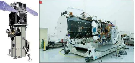
WorldView-3 (Fig. 1) is the last satellite of DigitalGlobe’s constellation of very high resolution satellites, which include IKONOS (launched September 24, 1999 - out of mission since 31.3.2015), QuickBird (October 18, 2001 - out of mission since 27.1.2105), WorldView-1 (launched September 2007), WorldView-2 (launched October 2009) and GeoEye-1 (launched September 6th, 2008). Table 1 shows a synthetic comparison of the different systems in terms of ground resolution, swath width, average revisit, bands, and overall geolocalization accuracy.
WorldView-3 was launched by DigitalGlobe (https://www.digitalglobe.com/) on August 2014, from Vandenberg Air Force Base in California. It collects images from an altitude of 617 km with a global capacity of 680,000 km2 per day. Ground resolution (ground sampling distance, GSD) is around 0.31 m for panchromatic images at nadir (0.34 m at 20° Off-Nadir), 1.24 m for multispectral images at nadir (1.38 m at 20° Off-Nadir), and 3.7 m for SWIR images at nadir (4.10 m at 20° Off-Nadir).
Figure 1. A rendered image of the WorldView-3 spacecraft (image credit: DigitalGlobe) and the spacecraft during AIT (Assembly, Integration and Test) phase (image credit: BATC).
The system carries an atmospheric monitoring instrument called CAVIS with 12 bands (desert clouds, aerosol-1, aerosol-2, aerosol-3, green, water-1, water-2, water-3, NDVI-SWIR, cirrus, snow) and a ground resolution of 30 m at nadir.
The swath width of 13.1 km at nadir coupled with very high scan acquisition rate (20,000 lines/second) for panchromatic images allows the acquisition of data for a large variety of applications such as land use and planning, telecommunications, infrastructure planning, environmental assessment, marine studies, mapping and surveying, civil engineering, mining and exploration, oil and gas, agriculture, etc.
Satellite WV-3 WV-2 WV-1
GeoEye-1
Ikonos Quick Bird GSD
(cm) 31 46 50 41 82 61
Swath Width
(km) 13.2 16.4 17.6 15.2 11.3 8
Average Revisit
(days) 1 1.1 1.7 2.6 3 2.5
Bands
Pan Pan
Pan
Pan Pan Pan 8MS
8SWIR 8MS 4MS 8MS 4MS CAVIS
CE90
3.5 m 3.5 m 4 m 5 m 3.5 m 23 m
Table 1. Comparison between some high resolution satellite systems.
A short revisit time can be achieved with large off-nadir angles (less than one day for large off-nadir angles, 4.5 days at 20 degrees off-nadir or less). The dynamic range is 11-bits per pixel for Pan and MS and 14-bits per pixel for SWIR. The The International Archives of the Photogrammetry, Remote Sensing and Spatial Information Sciences, Volume XLI-B1, 2016
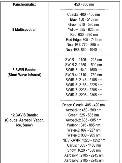
expected mission life is 7.25 years. WorldView-3 also collects shortwave infrared (SWIR) imagery in eight-bands, offered on a commercial satellite for the first time. A synthesis of the available bands is shown in Table 2.
Panchromatic:
Table 2. The bands of WorldView-3.
1.2 Geolocalization accuracy
WV-3 images are delivered with different pre-processing levels, radiometric corrections and geometric enhancement options that provide different levels of geometric accuracy (DigitalGlobe, 2013). One of the parameters able to provide an overall indication about the geolocalization accuracy is the circular error 90 at 90th percentile (CE90). This means that a minimum of 90 percent of the object points has a horizontal error less than the provided CE90 value. This index provides global information on the absolute geolocation accuracy. CE90 can be estimated with a comparison between the location of an object derived from the image and its true location on the Earth. The CE90 of WV-3 (3.5 m) is much larger than ground sampling distance (GSD = 0.31 m), resulting in a large discrepancy between image resolution and geolocalization accuracy. Similar considerations can be found for other VHR systems. Shows in Table 1 are the results for the different systems of DigitalGlobe’s constellation, resulting in an evident discrepancy between the achievable metric accuracy and the exterior orientation parameters provided with the images. In addition, CE90 does not take into account other error sources, like variable off-nadir angles and terrain effects, which could result in a worse metric accuracy. For instance, basic and standard products are based on a constant surface (a plane) used to approximate the Earth’s surface. In this case, some authors developed a modified version of the CE90 where these
additional effects are used to provide more information about the overall metric accuracy achievable before the ortho-rectification process (Crespi et al., 2015).
Different post-processing methods were developed to overcome the limitation of the provided direct orientation parameters. Usually, a set of ground control points (GCPs) measured by GPS is used to refine the initial RPCs, obtaining a set of corrections that can be assumed as biases in image space. This leads to an indirect orienta tion performed by the user with specific tools available in commercial software for satellite image orientation.
Nowadays, different sensor models are used to describe the relationship between the three-dimensional (3D) point position in object space (X, Y, Z) and the corresponding two-dimensional (2D) image point (x, y). Usually, exterior orientation parameters are provided via rigorous models (Poli and Toutin, 2012) or Rational Polynomial Coefficients (RPC, Fraser et al., 2002), which allow the rigorous model to remain confidential. In the case of WV-3 images, Rational Polynomial Coefficients are provided with an additional textfile which can be read and imported by most commercial software for high resolution satellite image processing (Envi, ERDAS, PCI Geomatica, etc.) The RPC camera model provides the relationships between image and object coordinates as follows:
= , ,, , ; = , , , , coordinates estimated from the measured line and sample coordinates:
= − �� �� �
(3)
= − �� �
The offset values are provided in the header of the RPC textfile. (X, Y, Z)are the corresponding object point coordinates in terms
The bias-compensated RPC camera model described in Hanley et al. (2002) is based on the hypothesis that errors in sensor orientation can be modelled as biases in image space for the very narrow field-of-view of the satellite line scanner, approaching a parallel projection. The method was tested on different kinds of high resolution satellite images (Dowman and Dolloff, 2000; Di et al., 2003; Aguilar et al., 2008). It provided sub-pixel results with a simple mathematical model based on an affine transformation (6 parameters) of the form:
+ + + = , ,, ,
(5)
+ + + = , ,, ,
where the coefficients and represent a translation in image space.
This means that three non-collinear GCPs are sufficient to estimate the 6 unknown parameters. On the other hand, a dense set of GCPs with a homogenous distribution provides an overdetermined system of equations which can be solved via least squares.
Practical experiments demonstrated that the correction of some satellite images could require the full set of affine parameters (e.g. QuickBird, Noguchi et al., 2004) or a simplified version based on 2 shifts ( and ), in which 1 GCP is sufficient (e.g. IKONOS, Fraser and Hanley, 2003).
The bias-compensated camera model can also be used in stereo or multi-image networks (Grodecki et al., 2003), where additional tie points are included in the model. 3D coordinates are provided by spatial intersection based on least squares. The case study presented in this paper is based on a single image, whose RPCs were refined with a set of 3D points and their corresponding 2D image coordinates.
2. DATASET DESCRIPTION
The bias-compensated RPC camera model was used to refine the RPCs of a WV-3 image provided by DigitalGlobe (https://www.digitalglobe.com/), which was acquired over Milan (Italy) on 15th Aug 2015. The image has an average metric resolution of 0.3 m, total max off nadir angle is 24.87°, and the covered area is 15.2 km × 20.5 km.
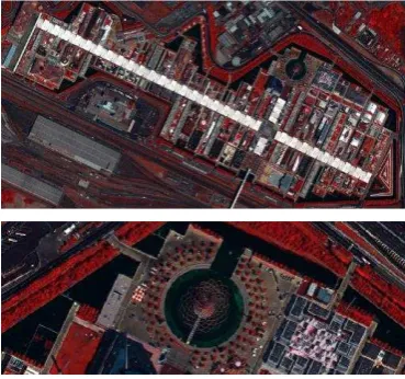
Fig. 2 shows a detail of the pan-sharpened product over the area of EXPO 2015, hosted in Milan in the Rho Fiera area.
Figure 2. Detail of the pansharpened image for the EXPO area.
Ground control points were measured with differential GNSS techniques using the new service of GNSS permanent stations of Lombardy and Piedmont regions: SPIN GNSS. The RTK survey provided coordinates in the reference system ETRF2000-RDN, 2008.0.
Points with a homogenous distribution were collected in three days (Figure 3). The precision was better than ±3 cm for both East (X) and North (Y) coordinates, and ±5 cm in elevation (h).
Figure 3. The set of points measured via RTK.
3. RESULTS
3.1 Estimation of correction parameters
The estimation of the bias-compensated RPC camera model was carried out with ERDAS Imagine, Exelis ENVI, Barista (developed by Cooperative Research Centre for Spatial Information (CRCSI), http://www.baristasoftware.com.au/) and an in-house package developed for scientific purposes. The algorithm implemented in the in-house software is based on a linear formulation of the form for:
[
… … … …]
[ ] = [
� , ,
� , , −
� , ,
� , , −
…
] (5)
for the full set of affine parameters, or the simplified model for the correction with two shifts:
[
… …] [ ] = [
� , ,
� , , −
� , ,
� , , −
…
] (6)
Table 3 shows the results for an analysis with 54 points used as GCPs and different software packages. A ground resolution of 0.3 m was used to convert least squares statistics (given in The International Archives of the Photogrammetry, Remote Sensing and Spatial Information Sciences, Volume XLI-B1, 2016
pixels) into metric units. As can be seen, the results with the full set of correction parameters are similar for ERDAS Imagine, Excelis ENVI and the in-house software, whereas Barista provided slightly better results. The correction model based on 2 shifts provided similar results (of about 0.7 m) to the full set of affine parameters, demonstrating that 2 shifts are sufficient for the Milan image.
The direct use of the provided RPC (see ERDAS and Barista) leads to an overall error larger than 2 m (using the overall RMSE = [(RMSE X)2 + (RMSE Y)2]1/2. Results with this configuration are well below the expected localization accuracy of WV-3 (CE90 = 3.5 m).
SW Correction RMSE X
(m)
RMSE Y (m)
ERDAS None 2.04 1.14
ERDAS Shift 0.75 0.78
ERDAS Affine 0.69 0.73
ENVI Affine(?) 0.69 0.73
Barista None 1.92 1.02
Barista Shift 0.71 0.72
Barista Affine 0.66 0.66
In-house sw Shift 0.75 0.78
In-house sw Affine 0.69 0.73
Table 3. Comparison between different software and correction models for the Milan dataset with 54 points used ad GCPs.
The RMSE values are directly provided by least squares statistics turned into metric units by taking into consideration ground resolution. Independent check points were not used in this test because the goal was the evaluation of different sw
packages able to handle orientation parameters of very high resolution satellite images. The results in table 3 show very similar results for the different software, further analysis are carried out only with ERDAS Imagine.
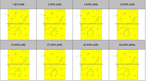
Table 4 shows the results with a correction model based on 2 shifts with different GCP and CP (check point) configurations derived from the original dataset of 54 points. Here, points were progressively set as check points to evaluate metric accuracy. The choice of the mathematical model with 2 parameters is motivated by the small improvement achieved with the full set of affine parameters. As can be seen, the achieved accuracy is about 0.8 m for both X and Y components. The value becomes quite stable after the use of only 3 – 4 ground control points for bias estimation, demonstrating that few GCPs are sufficient. Finally, a graphical visualization of point residuals (in terms of image coordinates) with different point configurations is shown in Fig. 4.
# GCP
# CP
GCP results CP results
RMSE X (m)
RMSE Y (m)
RMSE X (m)
RMSE Y (m)
1 53 - - 0.86 1.37
2 52 0.28 0.57 0.77 0.95
4 50 0.20 0.65 0.79 0.79
10 34 0.63 0.53 0.82 0.83
19 35 0.55 0.66 0.86 0.85
27 27 0.56 0.73 0.92 0.82
54 0 0.75 0.78 - -
Table 4. Results with ERDAS Imagine and different GCP and CP configurations. The correction model is based on 2 shifts.
1 GCP (shift) 2 GCPs (shift) 4 GCPs (shift) 10 GCPs (shift)
19 GCPs (shift) 27 GCPs (shift) 54 GCPs (shift) 54 GCPs (affine)
Figure 4. Schematic visualization of residuals with different control point (triangle) and check point (circle) configurations. The International Archives of the Photogrammetry, Remote Sensing and Spatial Information Sciences, Volume XLI-B1, 2016
It is important to mention that the previous results were obtained by removing some points from the original dataset, which is made up of 58 points. Indeed, large residuals mainly localized in the center of the image (which is also the center of the city) where found for 4 points. It is not clear why these additional 4 points gave a general worsening of metric accuracy: RMSE X = 0.94 m and RMSE Y = 0.77 m (overall RMSE = 1.21 m), estimated using the full dataset of 58 ground control points (Fig. 5 – left, blue circles indicate the 4 additional points). After removing these points from data processing, that are therefore assumed as additional check points, the computed values for GCP became: RMSE X = 0.75 m and RMSE Y = 0.78 m, overall RMSE = 1.07 m (Fig. 5 – right). On the other hand, the values for these 4 points used as check points are much worse: RMSE X = 1.59 m and RMSE Y = 2.94 m (RMSE = 3.34 m). This aspect will be investigated in the following section with the use of a geospatial database for accuracy evaluation.
Figure 5. Large residuals found for 4 additional points close to the center of the image.
3.2 Accuracy of the terrain-corrected image
Starting from the set of parameters computed using the set made up of 54 control points, a terrain-corrected image (i.e. an orthophoto) was generated with the digital elevation model SRTM30. Although the DEM has a spatial resolution (grid size) worse than WV3 pixel resolution, the city of Milan is a relatively flat area. This justifies the use of products with different spatial resolution.
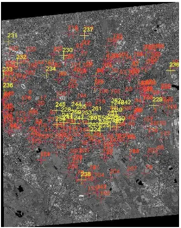
The terrain-corrected image (ortho-projected with a ground resolution of 0.3 m) was manually compared with the building layer of the geospatial database of the city of Milan (scale 1:1000). The analysis was carried out with more than 250 points, obtaining an overall RMSE of 1.21 m.
Fig. 6 shows the used points and their distribution. The points highlighted in yellow (mainly located close to the center of the image) exhibit the largest residuals. This result confirms the statistics computed in the previous section with check points measured via GNSS techniques (RTK). After removing these yellow points from the comparison, the overall geolocalization accuracy is defined by a RMSE of 0.76 m. This result is better than CP statistics and can be motivated by the simpler identification of building corners, instead of points measured via GNSS for which it was not often easy to identify the measured points in the image.
It is not clear why points close to the center of the image exhibit this error. A visual comparison between the vector layer and the orthorectified satellite image is shown in Fig. 7. The area is Piazza Duomo, i.e. the square in the center of the city. As can be seen, there is a clear spatial displacement.
Figure 6. Visualization of the points used for the comparison with the building vector layer. Points in yellow exhibit largest errors and are mainly located close to the center of the image (the center of the city).
Figure 7. The discrepancy between geospatial database and orthorectified image. Cathedral and square are located in the center of the image.
4. CONCLUSIONS
This paper presented the orientation results for a single WV-3 image collected over Milan. The use of a bias-compensated RPC camera model based on two shifts parameters improved geolocalization accuracy up to 0.7 m for both X and Y directions. The use of an affine model (6 parameters) did not provide significant improvements.
The comparison was carried out with a set of GCPs and CPs measured with RTK GNSS, as well as an independent evaluation between the terrain corrected image (orthophoto) and the geospatial database of the city (vector layer). Both tests confirmed a similar geolocalization accuracy. It should be mentioned that the original dataset of 58 points measured via RTK survey was reduced to 54 points, for which the expected geolocalization accuracy of these points is better than ±5 cm. 4 points were removed from the original dataset because of the large error in terms of point residuals. Similar results were obtained with the geo-corrected image compared to the building layer of the city (vector data), choosing elements close to the previous 4 points. These points are mainly located in the center of the image, i.e. the center of the city. The reason of this error is still not clear and will be investigated in future work.
ACKNOWLEDGEMENTS
The authors would like to thank DigitalGlobe for providing the WV-3 image over Mila and the Cooperative Research Centre for Spatial Information (CRCSI) for the demo version of Barista.
REFERENCES
Aguilar, M.A., F.J. Aguilar, and F. Agüera, 2008. Assessing geometric reliability of corrected images from very high resolution satellites, Photogrammetric Engineering & Remote Sensing, 74(12):1551–1560.
Ager, T.P., 2003. Evaluation of the geometric accuracy of IKONOS imagery. SPIE 2003 AeroSense Conference, Orlando, 21-25 April, 8 pages.
Di, K., Ma, R. & R. Li, 2003. Rational functions and potential for rigorous sensor model recovery. Photogrammetric Engineering and Remote Sensing, 69(1): 33-41.
Crespi, M., De Paulis, R., Pellegri, F., Capaldo, P., Fratarcangeli, F., Nascetti, A., Gini, R., Selva F., 2015. Mapping with high resolution optical and SAR imagery for oil & gas exploration: potentialities and problems. IGARSS 2015, 26-31 July 2015, Milan, Italy.
DigitalGlobe, 2013. Geolocation Accuracy of WorldView Products
Dowman, I. & J.T. Dolloff, 2000. An evaluation of rational functions for photogrammetric restitution. Int. Archives of Photogrammetry and Remote Sensing, 33(B3/1): 252-266.
Fraser, C.S., H.B. Hanley, and T. Yamakawa, 2002. 3D geopositioning accuracy of Ikonos imagery, The Photogrammetric Record, 17(99):465–479.
Fraser, C.S., and H.B. Hanley, 2003. Bias compensation in rational functions for Ikonos satellite imagery, Photogrammetric Engineering & Remote Sensing, 69(1):53–57.
Grodecki, J., and G. Dial, 2003. Block adjustment of high-resolution satellite images described by rational polynomials, Photogrammetric Engineering & Remote Sensing, 69(1):59–68. Hanley, H.B. & C.S. Fraser, 2001. Geopositioning accuracy of IKONOS imagery: indications from 2D transformations. Photogrammetric Record, 17(98): 317-329.
Hanley, H.B., Yamakawa, T. & C.S. Fraser, 2002. Sensor orientation for high-resolution satellite imagery. International Archives of Photogrammetry and Remote Sensing, Albuquerque, 34(1): 69-75 (on CD-ROM).
Noguchi, M., C.S. Fraser, T. Nakamura, T. Shimono, and S. Oki,
2004. Accuracy assessment of QuickBird stereo imagery, The Photogrammetric Record, 19(106): 128–137.
Poli, D., and Toutin, T., 2012. Review of developments in geometric modelling for high resolution satellite pushbroom sensors. The Photogrammetric Record, 27(137): 58-73.
Tao, V. & Y. Hu, 2002. 3D reconstruction methods based on the rational function model. Photogrammetric Engineering & Remote Sensing, 68(7): 705-714.
Barista, 2016. http://www.baristasoftware.com.au (accessed February, 2016)
ERDAS Imagine, 2016. http://www.hexagongeospatial.com/ (accessed February, 2016)
Exelis ENVI, 2016. http://www.exelisvis.com/ (accessed February, 2016)
DigitalGlobe, 2016. http://www.digitalglobe.com/ (accessed February, 2016)