WAVEFORM ANALYSIS FOR THE EXTRACTION OF POST-FIRE VEGETATION
CHARACTERISTICS
F. Pirotti a, *, A. Guarnieri a, A. Vettore a
a
CIRGEO, Interdepartmental Center for Research in Geomatics, 35020 Legnaro (PD) - Italy - (francesco.pirotti,
alberto.guarnieri, antonio.vettore)@unipd.it
Commission VII, WG VI/4
KEY WORDS: Full Waveform laser scanner, vegetation height distribution, airborne lidar survey
ABSTRACT:
Full-waveform is becoming increasingly available in today’s LiDAR systems and the analysis of the full return signal can provide additional information on the reflecting surfaces. In this paper we present the results of an assessment on full-waveform analysis, as opposed to the more classic discrete return analysis, for discerning vegetation cover classes related to post-fire renovation. In the spring of 2011 an OPTECH ALTM sensor was used to survey an Alpine area of almost 20 km2 in the north of Italy. A forest fire event several years ago burned large patches of vegetation for a total of about 1.5 km2 . The renovation process in the area is varied because of the different interventions ranging from no intervention to the application of re-forestation techniques to accelerate the process of re-establishing protection forest.
The LiDAR data was used to divide the study site into areas with different conditions in terms of re-establishment of the natural vegetation condition. The LiDAR survey provided both the full-waveform data in Optech’s CSD+DGT (corrected sensor data) and NDF+IDX (digitizer data with index file) formats, and the discrete return in the LAS format. The method applied to the full-waveform uses canopy volume profiles obtained by modelling, whereas the method applied to discrete return uses point geometry and density indexes. The results of these two methods are assessed by ground truth obtained from sampling and comparison shows that the added information from the full-waveform does give a significant better discrimination of the vegetation cover classes.
* Corresponding author. This is useful to know for communication with the appropriate person in cases with more than one autho r. 1. INTRODUCTION
Airborne LiDAR (or Airborne Laser Scanning - ALS) in the past ten years has seen rapid growth in both sensor technology and fields of application. Research on laser profilers started in the late nineties and a lot of interest was given to the forestry environment because of the ability of the laser pulse to penetrate canopy, returning ground hits, which are precious for digital terrain models (DTMs) extraction (Carson et al., 2004). Studies over the rate of penetration show that typical coniferous and deciduous forests allow 20-40% of the laser pulses to return ground hits in leaf-on conditions and as much as 70% in leaf-off conditions (Ackermann, 1999). This can occur because the size of the diffraction cone (Mallet and Bretar, 2009) can vary from a few centimeters up to one/two meters; thus the canopy area that is illuminated is large enough to have a significant amount of gaps which allow part of the laser energy to pass without getting reflected by leaves of branches, all the way to the ground, which is the element which causes the last reflection.
Discrete-return ALS systems provide data as 3D coordinates and intensity, commonly referred to as ―point cloud‖, by on-line processing of the return laser echo. If one laser pulse gets reflected by different surfaces along its path, interactions of the laser with the objects cause a return signal whose characteristics are a mixture derived from the different optical properties of the objects, the range and the incidence angle (Wagner et al., 2006).
Ranges from multiple returns are recorded depending on the sensor; two echoes (first and last) or multiple echoes (up to eight) can be recorded. Each sensor has a range resolution which describes the minimum distance required between objects, for separating two return echoes. This measure depends on the outgoing pulse duration and the group velocity, some ALS systems have a dead zone of up to 3 m (Wagner et al., 2008). Discrete-return sensors process the return echo waveform using fast yet simple algorithms like the Constant Fraction Discriminator criteria for defining a threshold for the identification of significant energy peaks (Thiel and Wehr, 2006).
Off-line processing of the waveform requires recording the full waveform of the return echo by means of a digitizer which samples the return energy at certain time intervals usually from one to several nanoseconds. To this day a significant amount of tests have been conducted on waveform data from spaceborne
and airborne sensors. NASA’s GLAS sensor, mounted on
IceSAT satellite provided freely downloadable full waveform data for several years before recent mission dismissal. The main objective was the estimation of the thickness and dynamics of the polar ice-sheet (Zwally et al., 2002), but its large-footprint (~65 m) waveform information was also used also for extracting vegetation structure (Harding and Carabajal, 2005), ground cover classification (Pirotti, 2010) as well as direct canopy International Archives of the Photogrammetry, Remote Sensing and Spatial Information Sciences, Volume XXXIX-B7, 2012
mapping (Simard et al., 2008) and above-ground biomass extraction (Lefsky et al., 2005). A high-altitude airborne sensor tested was SLICER, providing ~10 m footprints at ~5000 m altitude. Harding et al. (2001) proved that canopy height profiles can be extracted from waveform data with correlation (R2) values up to 0.75 can compared with ground truth. Lefsky et al. (2005) used SLICER data to estimate above ground biomass (AGBM) over different biomes, reaching correlation (R2) values up to 0.85.
A strategy of processing waveform is to attempt for an improvement in peak detecting in the post-processing phase. Several methods have been tested and results show that the Generalized Gaussian fitting method gives best results (Chauve et al., 2007). Improved peak detection increases the number of significant returns obtained from a survey. Tests have shown that the number of returns – thus point density – can be increased by a factor of two compared to conventional discrete-return data (Reitberger et al., 2009). Point clouds with high densities ( 10 point/m2) are necessary for extracting metrics which use the distribution of 3D positions and intensities (Reitberger et al., 2009) for the identification of single trees and tree structure.
Metrics which use all the information obtainable from an ALS survey have also been tested on large footprint (Drake et al., 2002) and small-footprint surveys. The objective of this paper is to extract information on low vegetation (renovation) by discrimination of terrain from low vegetation returns.
2. MATERIALS AND METHODS 2.1 Study area and ALS survey
The survey was done the 20th of June 2011 with a helicopter carrying Optech’s ALTM 3100 sensor and a Rollei AIC modular P45 digital metric camera. The surveyed area is a region whose area is approximately 2.70 km2, located in the northwest part of Italy. The region of interest (ROI) for this study is a smaller
portion (center at 7°29’54‖ longitude 45°46’18‖ latitude at
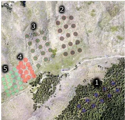
WGS84 datum). Part of the ROI encompasses and area which endured a severe fire event in 2005 which caused the destruction of the forest stand. Figure 1 shows the ROI with circular sample plots on five the five sectors which were tested for variability in vegetation characteristics.
Figure 1. ROI with the five sectors with circular sample plots
Characteristic Value
Vehicle Helicopter
Sensor Optech ALTM 3100
Date of survey June 20 2011
Mean relative flight height 525 m above ground
Scan angle* 21.5°
Scan frequency* 71.5 KHz
Output Datum ETRS2000 (2008) – WGS84 *Calculated directly from the output data
Table 1. Characteristics of the survey flight.
2.2 ALS data
In the text the term ―waveform‖ will be used to indicate amplitude as a function of time, specifically a vector of energy values sampled at 1 ns intervals. The length of the vector depends on the number of sampled energy values, which, in the
case of Optech’s waveform file format, is a variable number for the return echo. In the case of the outgoing pulse (T0), the energy is sampled constantly every 1 ns for 40 ns thus the T0 waveform is recorded in the NDF file using 40 samples. As can be seen in figure 2 the maximum value does not always correspond with the same sample time..
Figure 2. Plot of eight waveforms of the outgoing pulse.
2.3 Waveform recording format
All laser scanner data were stored by the system in Optech’s
waveform data file formats, which consist in four types of files. To process the waveform the following files were necessary: - NDF file, where the recorded waveform data are stored consisting of variable length records, each of which hold the following information relative to one laser pulse: the GPS timestamp, the outgoing pulse waveform and up to 7 significant segments of the corresponding return echo waveform. The NDF data are divided into frames, each containing 16838 records. - IDX file, which is an index, relating starting and ending GPS timestamps of a specific frame in the NDF file.
- CSD file holds information on trajectory, thus the position and orientation of the vehicle at each laser pulse, as well as scan angle and range of up to four returns.
- DGT file holds the index between frame start time and CSD record number.
2.4 Sampling design
The ROI was divided into 5 sectors with different characteristics in terms of forest cover and renovation technique; each area was sampled with circular plots of 12.6 m radius, 500 m2 (figure 1). The characteristics for each area and the number of plots are reported on the table below.
Sector Cover N° of samples
Table 2. Characteristics of the four test sectors.
The samples in the ROI where chosen with specific care of leaving out any surface which does not have a vegetation cover, to limit variability of the geometry and radiometry of the return echo, since, as it is described in literature (Jutsi and Stilla, 2003) there is significant variability even between different elements inside an urban environment.
2.5 Waveform extraction and analysis
The process for extracting the waveform data was done by implementing custom routines developed in c++ language which have been integrated in a tool with graphical user interface. This software is in very early development stages and is work in progress; anyone interested is welcome to contact the author for testing purposes. The objective of the software is to bundle methods for processing waveforms directly and for exporting
waveforms to more common formats such as ASPRS’ LAS 1.3
or future open standards.
The routine requires a shapefile with points representing the center of each sample plot, the radius of the plots and the folder path were all of the files are stored. It then proceeds in reading the plot coordinates, and filling a container for each sample with the pulses falling inside the sample area. Each pulse is then linked to the corresponding waveform data using the GPS timestamp to search the waveform file (see section 2.3).
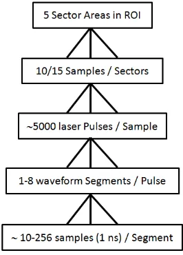
Figure 3. Plot of eight waveforms of the outgoing pulse.
Figure 3 shows a scalar relationship from the ROI down to the single 1 ns sample in the waveform segment.
The position in 3D space of each return sample at time t in the waveform segment can be calculated with the following: the sensor position, the sensor orientation, the pulse scan angle and the time interval (tn) between the beginning of emitted pulse (T0) and the beginning of the nth return echo waveform segment
coordinates of the sensor center, and Rs is the range of the first waveform sample.
The range R(t) is calculated using the speed of the laser pulse and the time interval between the maximum value of the T0 pulse (see figure 2) and the first sample over the baseline of the return waveform segment Tn:
where P is atmospheric pressure in mbar ant T is air temperature in degrees Celsius.
The method reported above was used to fill a voxel grid with 0.3 m resolution with information on the waveform data. The range was calculated for each waveform data which was significantly above the baseline of the return signal; an empirical value of 5 digitizer counts was used as threshold. This means that a surface which causes a reflection will imprint a high value in the voxel it falls.
The voxel grid is then used to extract statistical information on vegetation height and density over the whole sample, and successively over the whole sectors. The Kolmogorov-Smirnov two-sample test (K-S) is a non-parametric test that is sensitive to both the shape and location of peaks within the distribution and was used to compare between samples in the same sector and between samples over different sectors to check if inter- and intra- variances are significantly different thus leading to the possibility of using the method to discriminate areas with different vegetation structure.
3. RESULTS AND DISCUSSION
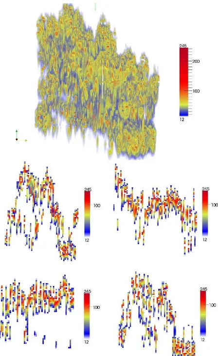
This method sample the waveform information in 3D space, and will be the basis of further work for vegetation analysis. It is different from more common methods which use fitting of waveforms to discriminate between returns and use peak values to have a dense point cloud with width and amplitude information. In this case we base our method on statistics on the voxel grid, which overrides any signal analysis step necessary for determining the point in space which causes the reflection. In this case the return waveform from a reflecting surface will not supply information to a single point in space or to a single voxel, but will be supplying information to many voxels along its path. The resolution of 0.3 m was chosen empirically as it is a space which can include ~2 successive samples. A bigger voxel size would be less discriminate, whereas a smaller voxel size would not improve results, but increase threefold the size of the files. As can be seen in figure 4, results can visually report vegetation structure. Table 3 reports the results of the K-S test over the distribution of metrics extracted from the voxel grid, showing International Archives of the Photogrammetry, Remote Sensing and Spatial Information Sciences, Volume XXXIX-B7, 2012
that the differences between samples in different sectors is significant over sector 1 (forest) and the other sectors. Sector 3 is also significantly different from the other sectors except sector 2. This can be explained on the fact that the area in sector 3 has stems of deadwood standing, thus the height distribution is different from the other sectors, where all stems were cut down. The method was not able to discriminate between sectors 2, 4 and 5. The low vegetation present and the sample area size do not bring enough height variance between them for discrimination. A solution could be to use smaller sample plots over more representative spots, avoiding the inclusion of a large percent of bare ground in the plot. A stratified sampling procedure using image interpretation could be used to segment an image masking the ground area.
S1 S2 S3 S4 S5
S1 - 0.56* 0.46* 0.43* 0.52*
S2 - 0.36 0.19 0.12
S3 - 0.41* 0.47*
S4 - 0.11
S5 -
*Indicates a significant difference in distributions at = 0.05 Table 3. Characteristics of the four test sectors.
Figure 4. Top – 3D view of plot without ground returns – the scale reports the intensity in 8 bit scale. Bottom - four slices
from the voxel grid reporting digitizer counts of waveform.
Another factor to consider is that the sampling of the waveform occured with a nominal threshold which was chosen according to the observed values. This was possible because we worked on a single survey and thus the survey characteristics which influence the outgoing energy for every pulse – thus the return energy loss – where relatively constant (relative flying height, pulse frequency). A more objective method would be to calculate only the segment with Full Width at Half Maximum (FWHM) criteria.
4. CONCLUSIONS
The results are part of a more in-depth investigation for evaluating methods for discriminating low vegetation distribution over land for defining the effect of re-forestation methods in a broader ongoing project which investigates vegetation dynamics in areas which have been part of a severe fire event. A positive result over the sampled areas will enable to apply the method and evaluate results over larger areas to test for robustness. The proposed modifications mentioned in the discussion will be applied to test for improved results. The final objective is to provide a method to segment 3D space into significant information using waveform data.
5. ACKNOWLEDGEMENTS
This work is part of the CPDA097420 project funded by the University of Padua: "Disturbi naturali in foreste alpine: approccio multiscala e applicazioni LiDAR", scientific coordinator prof. Emanuele Lingua.
REFERENCES
Ackermann, F. 1999. Airborne laser scanning—present status and future expectations. ISPRS Journa l of Photogra mmetry a nd Remote Sensing 54(1), pp. 64– 67.
Carson, W.W., Andersen H-E., Reutebuch, S.E., McGaughey R.J. 2004. Lidar Applications in Forestry: an Overview. In:
ASPRS Annua l Conference Proceedings, May, Denver,
Colorado.
Chauve A., Mallet C., Bretar F., Durrieu S., Pierrot-Deseilligny M., Puech W. 2007. Processing Full-Waveform LiDAR Data: Modelling Raw Signals. In: Proceedings of the “Laser
Scanning 2007 and SilviLaser 2007” 2007. Espoo, Finland, September 2007, pp. 102-108.
Drake, J.B., Dubayah, R.O., Clark, D.B., Knox, R.G., Blair, J.B., Hofton, M.A., Chazdon, R.L., Weishampel, J.F., Prince, S. 2002. Estimation of tropical forest structural characteristics, using large-footprint LiDAR . Remote Sensing of Environment
79, pp. 305-319.
Harding, D.J., Lefsky M.A., Parker, G.G., Blair, J.B. 2001. Laser altimeter canopy height profiles methods and validation for closed-canopy, broadleaf forests. Remote Sensing of
Environment 76, pp. 283-297.
Harding, D.L., Carabajal, C.C. 2005. ICESat waveform measurement of within-footprint topographic relief and vegetation structure. Geophysica l Resea rch Letters 32, L21S10. International Archives of the Photogrammetry, Remote Sensing and Spatial Information Sciences, Volume XXXIX-B7, 2012
Jutzi, B., Stilla, U. 2003. Laser pulse analysis for reconstruction and classification of urban objects. Interna tiona lArchives of Photogra mmetry, Remote Sensing a nd Spa tia l Informa tion Sciences 34 (Part 3/W8), pp. 151-156.
Pirotti, F. 2010. IceSAT/GLAS Waveform Signal Processing for Ground Cover Classification: State of the Art. Ita lia n Journa l of Remote Sensing 42(2), pp. 13-26.
Lefsky, M.A., Harding, D.J., Keller, M., Warren, Cohen, B., Carabajal, C.C., Espirito-Santo, F.E., Hunter, M.O., de Oliveira, R. 2005. Estimates of Forest Canopy Height and Aboveground Biomass using ICESat. Geophysica l Resea rch Letters 32, L22S02.
Lefsky, M.A., Hudak, A.T., Cohen W.B., Acker, S.A. 2005. Geographic variability in LiDAR predictions of forest stand structure in the Pacific Northwest. Remote Sensing of
Environment 95, pp. 532-548.
Mallet, C., Bretar, F. 2009. Full-waveform topographic LiDAR: State-of-the-art. ISPRS Journa l of Photogra mmetry a nd Remote Sensing 64(1) , pp. 1-16.
Reitberger, J., Schnorr, C., Krzystek. P., Stilla, U. 2009. 3D segmentation of single trees exploiting full waveform LIDAR data. ISPRS Journa l of Photogra mmetry a nd Remote Sensing
64, pp. 561-574.
Simard, M., Rivera-Monroy, V.H., Mancera-Pineda, J-E., Castaneda-Moya, E., Twilley, R.R. 2008. A systematic method for 3D mapping of mangrove forests based on Shuttle Radar Topography Mission elevation data, ICEsat/GLAS waveforms and field data: Application to Cienaga Grande de Santa Marta, Colombia. Remote Sensing of Env. 112, pp. 2131-2144.
Thiel, K., Wehr, A. 2004. Performance and capabilities of laser scanners - an overview and measurement principle analysis.
Interna tiona l Archives of Photogra mmetry, Remote Sensing a nd Spa tia l Informa tion Sciences 36, pp. 14-18.
Thomas, R. 2002. ICESat’s laser measurements of polar ice, atmosphere, ocean, and land. J. Geodyn. 34(3–4), pp. 405–445.
Wagner, W., Ullrich, A., Ducic, V., Melzer, T., Studnicka, N. 2006. Gaussian decomposition and calibration of a novel small-footprint full-waveform digitising airborne laser scanner. ISPRS Journa l of Photogra mmetry a nd Remote Sensing 60(1) , pp. 100-112.
Wagner, W., Hollaus, M., Briese, C., Ducic, V. 2008. 3D vegetation mapping using small-footprint full-waveform airborne laser scanners. Interna tiona l Journa l of Remote Sensing 29, pp. 1433-1452.
Zwally, H.J., Schutz, B., Abdalati, W., Abshire J., Bentley, C., Brenner, A., Bufton, J., Dezio, J., Hancock, D., Harding, D., Herring, T., Minster, B., Quinn, K., Palm, S., Spinhirne, J.,