Water balance, transpiration and canopy conductance
in two beech stands
A. Granier
a,∗, P. Biron
b, D. Lemoine
aaUnité d’Ecophysiologie forestière, INRA Centre de Nancy, F54280 Champenoux, France bCEREG, Université de Strasbourg, 3 rue de l’Argonne, F67083 Strasbourg Cedex, France
Received 2 November 1998; received in revised form 18 October 1999; accepted 21 October 1999
Abstract
Measurements of sap flow, vapour fluxes, throughfall and soil water content were conducted for 19 months in a young beech stand growing at low elevation, in the Hesse forest. This experiment is part of the Euroflux network, covering 15 representative European forests. Study of the radial variation of sap flow within tree trunks, showed a general pattern of sap flux density in relation to the depth below cambium. Among-tree variation of sap flow was also assessed, in order to determine the contribution of the different crown classes to the total stand transpiration. Stand sap flow and vapour flux, measured with eddy covariance technique, were well correlated, for half hourly as well for daily values, the ratios of the fluxes for both averaging periods being 0.77. A strong canopy coupling to the atmosphere was found, omega factor ranging between 0.05 and 0.20 relative to the windspeed. Canopy conductance variation was related to a range of environmental variables: global radiation, vapour pressure deficit, air temperature and soil water deficit. In addition to the effect of radiation and of vapour pressure deficit often found in various other tree species, here beech exhibited a strong reduction in canopy conductance when air temperature decreased below 17◦C. The model of transpiration was calibrated using data measured in the Hesse forest and
applied to another beech stand under mountainous conditions in the Vosges mountains (east France). Measured and modelled stand transpiration were in good agreement. ©2000 Published by Elsevier Science B.V. All rights reserved.
Keywords:Sap flow; Transpiration; Soil water content; Canopy conductance; Model;Fagus sylvatica
1. Introduction
Analytical studies of forest ecosystem functioning, and modelling of fluxes are of basic importance (see Tenhunen et al., 1998), because they constitute key data sets that are used for parameterisation of larger scale models, from watershed (hydrology) to the global scale (predicting weather and climate change), especially if those experiments cover several years, taking into account inter annual variation due to
cli-∗Corresponding author. Tel.:+33-383-3940-41; fax:+33-383-3940-69.
mate. There is an increasing interest in water and carbon fluxes at the canopy–atmosphere interface, due to the uncertainty linked with the perspective of cli-mate change. Forests cover large areas and therefore have a major contribution to total energy and mass fluxes. On the other hand, management of forests is much less intensive than management of agricultural crops. Therefore, forests will be more directly in-fluenced by the variations of climate. The European Union initiated the large scale programmeeuroflux
(‘Long term carbon dioxide and water vapour fluxes of European forests and interactions with the climate system’) to study the interactions between forests
and the atmosphere, constituting a framework of 15 experimental sites located in various climatic zones, in 10 different European countries. The programme
eurofluxis aiming at quantifying energy, water and
carbon dioxide fluxes over forests stands representa-tive of European forests, using eddy covariance (EC) as a common technique. A major objective is to derive parameters describing forest–atmosphere interface properties that can be used in larger scale models.
One of the tree species selected for theeuroflux
programme, beech (Fagus sylvatica L.) covers large areas in Europe, extending from south England, France and north Spain in its western limit to Poland and Romania in the east. Latitudinal extension ranges from south Sweden to north Italy and Greece. In its northern area, beech is mainly found at low elevations, while in the southern part of Europe it is located at higher elevations (Tessier du Cros, 1981); in France, beech covers about 13 000 km2and plays an important eco-nomic and recreative role.
The present study took place in a young beech stand growing in the east of France, combining tech-niques working at different spatial and temporal scales. In particular, we combined eddy covariance with sap flow and classical water balance measurements over a 2-year period.
This work is aiming at a quantification of the differ-ent water and energy fluxes in the beech ecosystem, focusing on tree transpiration and on total evapotran-spiration. The use of sap flow measurements allows the analysis of the variability in tree transpiration within the experimental plot, and to quantify the contribution of the different crown status to the total water flux. In this paper, tree transpiration, estimated from sap flow measurements, is compared to total evapotranspira-tion. Environmental and physiological control of stand evapotranspiration is then assessed using the variation of canopy conductance which is derived from climatic variables and from transpiration measurements. A big leaf model of beech transpiration, including the ef-fects of radiation, vapour pressure deficit, air temper-ature and water stress, is parameterised. In a next step, this model is applied to another beech stand, differing in age, structure and site conditions, in order to anal-yse to what extend transpiration differs between beech forests, and to assess the possibility of a more general use of the model. This work is aiming at: (1) quantify-ing the different fluxes of water in the beech
ecosys-tem, (2) analysing stand evapotranspiration in relation to climate, soil water content and tree phenology, con-centrating especially on within and among-tree vari-ation in sap flow, and on stand transpirvari-ation mecha-nisms, (3) deriving from the water flux measurements tree canopy conductance to water vapour, that can be extrapolated to other sites under different environmen-tal conditions, and (4) validating a model of stand transpiration in a second beech stand differing in age, structure and environmental conditions.
2. Materials and methods
2.1. Sites and stands
The experimental plot was located in the state forest of Hesse, France (48◦40′N, 7◦05′E, elevation 300 m),
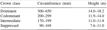
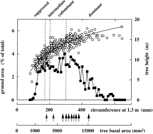
which was mainly (90%) composed of beech. Other tree species (about 10% of the ground area) are Carpi-nus betulus L., Betula pendula (Roth), Quercus pe-traea(Matt.), andLarix decidua(Mill.). Due to canopy closure, understorey vegetation was very sparse and its contribution to the water balance was neglected in this study. Trees were on an average 30 years old when the study started, stand density was 3800 stems ha−1, and basal area 19.6 m2ha−1. Average tree height and circumference (at 1.3 m) were 12.7 m and 227 mm, respectively. The experimental plot covered 0.6 ha; it was located in the central part of a 65 ha area homo-geneous, naturally established beech forest, ranging from ca. 10 to 16 m average height. Stem distribution in the plot is presented in Fig. 1. It shows an asym-metrical distribution, the smallest stems being much more numerous. Four tree classes were distinguished according to the crown characteristics (Table 1).
Three towers were installed: one (18 m height) was used for eddy covariance and microclimate
measure-Table 1
Circumference and height ranges of the four crown classes in the beech stand
Crown class Circumference (mm) Height (m)
Dominant 300–650 14.0–18.2
Codominant 200–299 11.9–14.0
Intermediate 170–199 11.0–11.8
Fig. 1. Frequency of stem circumference at height of 1.3 m (squares) and tree height (open circles) in the Hesse forest. Vertical black arrows indicate circumference and basal area of the trees equipped with sap flow meters in 1996 and 1997. Grey arrows are for trees measured only in 1997.
ments, the two other (15 m) for ecophysiological mea-surements. A hut containing the data acquisition sys-tems was located near the first tower. 60 sub-plots were delimited for geostatistical studies of soil and of vegetation. Nine of them were used for soil res-piration measurements and 12 other for dendrometric measurements (growth, height).
The soil type was intermediate between a luvisol and a stagnic luvisol. Clay content ranged between 25 and 35% within 0–100 cm depth, and was about 40% below 100 cm. Most of the root biomass was located between 0 and 40 cm depth, however minor roots (di-ameter<1 mm) were observed down to 150 cm depth in the soil (E. Lucot, personal communication). An-nual precipitation was 820 mm, average anAn-nual tem-perature 9.2◦C.
Some of the results obtained in the Hesse forest were compared to measurements performed in an older beech stand growing under mountainous condi-tions, in which sap flow and climate were recorded for 1 year, in 1995. This stand was located in the Aubure forest (Strengbach watershed, in the Vos-ges mountains, France, 48◦12′N, 7◦15′E), at 1000 m
elevation on a sandy soil characterised by a poor
mineral content and a low extractable soil water (ca. 100 mm). Average tree height was 22.5 m, trees were 120 years old, and stand density was 429 stems ha−1.
A more detailed description can be found in Biron (1994).
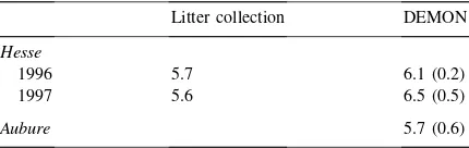
2.2. Leaf area index
Leaf area index (LAI) was estimated by means of two independent methods. Litter was collected during fall using forty-two 0.25 m2-square litter traps. Dry
Table 2
Maximum leaf area index (in m2m−2) at the two experimental sites, as estimated by litter collection and by DEMONa
Litter collection DEMON Hesse
1996 5.7 6.1 (0.2)
1997 5.6 6.5 (0.5)
Aubure 5.7 (0.6)
aStandard deviation is indicated in brackets.
These estimates of LAI are presented on Table 2. The seasonal time course of surface area index (SAI) was assessed from the measurement of global radiation absorbed by the canopies, using the Beer–Lambert law and the LAI (litter). The extinction coefficient was estimated as 0.40. Time course of SAI was calcu-lated on a daily time scale to reduce the effect of light distribution heterogeneity.
2.3. Throughfall, stemflow and soil water content
Forty-two standard raingauges were disposed on a grid over the experimental plot during the grow-ing season 1997, allowgrow-ing measurements of cumu-lated throughfall every 7 days. Throughfall was also measured automatically with two linear collectors (5.66 m×0.17 m), each one being connected to a
tipping bucket raingauge (ARG 100, Campbell Ltd., UK) and the data was recorded every 30 min. Because rainfall interception was calculated from throughfall as measured with the two automatic devices, we first calibrated them against measurements obtained from the 42 raingauges, for ten 1–7 day periods, each in-cluding at least one rain event. Throughfall from the two automatic systems was on average 4% lower than that measured with the 42 raingauges (r2=0.97). A
correction coefficient of 1.04 was therefore applied on half-hourly data obtained with linear collectors to calculate actual throughfall. Gross rainfall was mea-sured with an automatic raingauge (Campbell, ARG 100, UK) located above the canopy, at 17.5 m height on the central tower. Because this raingauge may be influenced by wind, there could be some bias in the gross rainfall measurements and in rainfall intercep-tion estimates.
Spiral channels disposed around the trunks con-nected to reservoirs allowed stemflow measurement
on seven trees of various circumference (ranging between 130 and 560 mm). Stemflow was measured every week, hence cumulating one or several rain events, during 6 months in 1997.
Soil water content was measured weekly using two techniques. During the years 1996 and 1997, volumet-ric water content (θNP) was measured with a neutron
probe (NEA, Denmark) in eight aluminium access tubes: six tubes were 1.6 m long, and two tubes were of 2.6 m length. Five of these tubes were installed nearby the central part of the plot (Zone 1), while the other three were in the eastern part (Zone 2). This distinction was based on visual observation of soil cores showing a spatial variation in the soil characteristics within the experimental plot: in the central part, where most of the ecophysiological measurements were performed, soil was deeper and contained less clay (27.9%) than in the eastern part (34.3%). In 1997, a TDR device (Trase system, Soil Moisture, USA) was additionally used to measure soil water content (θTDR) in the
superficial soil levels from twelve 0.4 m-long wave guides. A good agreement was found between neu-tron probe and TDR, when averaging humidity mea-surements from the neutron probe over the 0–0.4 m depth is
θNP=1.10θTDR (1)
From the distribution profiles of water content over 2.6 m soil depth, we calculated relative extractable water (θe) in the soil as the ratio of actual extractable
water to maximum extractable water (Black, 1979), the latter term being equal to the difference between maximum and minimum soil water content. Maximum water content was evaluated as the average of wettest profiles measured during winter and early spring. Min-imum water content was estimated from water reten-tion curves established at –1.6 MPa between−0.1 and
–1.2 m.θe varies between 0 (soil dry) and 1 (at field
capacity).
2.4. Sap flow and wood water content
i.e. the sap flow per unit of sapwood area. In 1996, seven trees were measured continuously; in 1997, 10 trees. In 1996, as most of the trees equipped with sap flow meters were of medium or large circumference (C1.3> 250 mm), a complementary sample of five
trees of which the circumferences ranged from 130 to 240 mm was measured (from 11 July to 23 Septem-ber 1996) to assess the dependence of Fd on tree size.
Calculation of sap flow per tree and on a stand basis is based upon sapwood area of the trunk. Unfortunately, in beech, the visual distinction be-tween sapwood and heartwood is impossible. There-fore, additional sap flow experiments were conducted during the 2 years. In three trees, radial variation of
Fd was assessed using a set of five 10 mm long
sen-sors inserted at increasing depth (0–50 mm) below the cambium, thus measuring sap flux density within 10 mm wide concentric annulus of sapwood. These measurements were carried out during 1–2 month periods during the vegetation period, resulting in a general relationship between relative sap flux density and depth below the bark. This allowed derivation of a function relating total tree sap flow to the standard measurements of sap flux densities in the first 20 mm of sapwood.
Radial variation of wood water content in the trunk was assessed as an additional source of information on the sapwood extent in the trunk. Cores were taken from the trunks of 20 trees (at 1.3 m height) around the experimental plot among various circumferences, varying in from 240 to 360 mm. Cores were cut in 5 mm long subsamples, on which fresh and dry weight were measured in order to calculate wood moisture content, that was expressed in mass of water per unit of volume.
Trees to be equipped with sap flow meters were se-lected randomly within sapwood classes, and hence within the basal area classes, having the highest contri-bution to the stand sap flow (see Fig. 1). For instance, the biggest trees (C1.3> 500 mm) were not measured,
even if they could exhibit high sap flow rates, because they represented only a small proportion of the stand sapwood area.
Sap flow measurements performed throughout the vegetation period in individual trees were scaled to stand level using sapwood area distribution, as de-scribed in Granier et al. (1996a). Stand sap flow (ET)
was calculated as:
ET=ST6piFDi (2)
whereSTis the stand sapwood area per unit of ground
area (m2m−2),p
i is the proportion of sapwood in the
classi, andFDi is the average sap flux density in the
classi.
2.5. Eddy covariance
Water vapour and carbon dioxide fluxes were mea-sured at 18 m height, i.e. 5 m above the mean tree height, from a tower installed in the middle of the plot. The three axis components of windspeed were mea-sured with a 3-D sonic anemometer (Solent model R2, Gill, UK). Air was drawn from the top of the tower to a hut through a 30 m long 4 mm diameter PTFE tub-ing. The inlet, equipped with a 0.2mm filter, was
lo-cated at the base of the 3-D anemometer. Air flow rate was 10−4m3s−1. Water vapour and carbon dioxide
concentration were measured with a LI-6262 IRGA analyser (Li-Cor, USA). Scanning of windspeed and gas concentration was made at a frequency of 10 Hz. Edisol software (Moncrieff et al., 1997) was used to process on-line sensible heat, carbon dioxide and wa-ter fluxes, following the recommendations made by Aubinet et al. (1999). This software calculates the 3-D coordinate rotation and the time lag correction due to the tube length. This time lag was on average equal to 3.8 s for CO2and 4.3 s for H2O. The time constant
used for the digital filter was 200 s.
Eddy covariance measurements started on 20 May 1996. On 31 December 1996, 160 days of opera-tion were available, i.e.70% reliable data. Throughout
elementary terms (latent, sensible, soil heat flux, heat storage) was equal to 88% of net radiation.
2.6. Climate
The following instruments were installed above the stand at 17.5 m height: a net radiometer (REBS, Seattle, USA), a global radiometer (Cimel, France), a ventilated psychrometer (INRA, France, with Pt 100 temperature sensors), a raingauge (Campbell ARG 100, UK), and a switching anemometer (Vector Instruments, UK).
Within and below the canopy, global radiation was measured at 1, 8, 10 and 12 m height using 0.33 m long linear pyranometers (INRA, France). Tree pyra-nometers were installed at 1 m height in order to have a better estimate of the radiation reaching the soil sur-face. Trunk and branch temperatures were measured at 1.5, 6, 8 and 10 m in one tree with copper–constantan thermocouples, soil heat flux with two heat flux trans-ducers (REBS, Seattle, USA) placed at−5 cm in the
soil, soil temperature (with copper–constantan ther-mocouples) at−10 cm (five replicates) and one
verti-cal profile (−5,−10,−20,−40,−80 cm) in a central
plot. Data acquisition was made with a Campbell (UK) CR7 datalogger at 10 s time interval, 30 min averages were calculated and stored.
2.7. Canopy conductance
Canopy conductance for water was calculated by inverting the Penman–Monteith equation in the same way as in Gash et al. (1989). In the present work, we estimated: (1) total canopy conductance (gcT) from
water vapour flux, and (2) tree canopy conductance (gc) from scaled sap flow measurements on a ground
area basis (see Köstner et al., 1992, Granier and Lous-tau, 1994, Granier and Bréda, 1996, Granier et al., 1996b). Aerodynamic conductance (ga) was estimated
from windspeed using the equation:
ga= k
is the windspeed at heightz.
For calculating tree canopy conductancegc, night
data and periods of rainfall were eliminated, as well as early morning and late afternoon data when radiation, air vapour pressure deficit and sap flow were close to zero, increasing the relative inaccuracy in canopy con-ductance calculation. We distinguished between dry and wet canopy conditions for computinggcT.
3. Results
3.1. Throughfall, stemflow, rainfall interception and soil water content
The relationships relating throughfall and stemflow to incident rainfall, shown in Fig. 2, were used to com-pute rainfall interception. No clear relationship be-tween stemflow and stem diameter was detected (data not shown). Stemflow was observed only when rain-fall exceeded the threshold of 2 mm, reflecting the condition when branches and trunks were wet enough to allow water to flow down the bark surface. The quite low scattering of data for throughfall is due to the analysis of individual rain events instead of cumu-lated rain. For rainfall events of 5, 10 and 15 mm, ratio of intercepted water to incident rainfall reached 30.0, 26.6 and 25.3%, respectively. Over the whole grow-ing season in the Hesse forest, this ratio was 25.3 and 26.8% in 1996 and 1997, respectively, and 23.4% in the Aubure forest. On an average, during the vegeta-tion period, throughfall and stemflow represented 26 and 5% of the incident rainfall, respectively.
During summer 1996, drought developed progres-sively and water stress lasted from the end of July to the end of October. Water stress was defined whenθe
Fig. 2. Top: relationship between stand throughfall,Th, and gross rainfall,P, each data point corresponding to one rain event (n=57). Data were obtained from two automatic linear collectors previ-ously calibrated against 42 standard raingauges standing on the soil. Bottom: relationship between stand stemflow and gross rain-fall, obtained from scaled measurements performed with spiral collectors installed on seven trees of various circumference. Each data point (n=12) is cumulated over 1 week.
extraction occurred was 1.6 m versus 0.8 m, in Zone 1 and Zone 2, respectively. Two phases in dehydration can be observed: first, the decrease in soil water con-tent occurred between soil surface to 1.0 m depth (see curves of 24 May, 18 and 28 June in Fig. 3a), then, as root absorption continued, water was withdrawn in the deeper soil layers, (from 1.0 to 1.6 m in the period from 28 June to 5 September). In Zone 2, water ab-sorption occurred only within the 0–0.8 m soil layer. Maximum extractable water was calculated as the dif-ference between maximum and minimum measured water content. It ranged between 100 and 200 mm and was on average 185 and 130 mm in Zone 1 and Zone
2, respectively. TDR measurements performed in the superficial soil layer (0–0.4 m) confirmed these obser-vations (data not shown).
3.2. Transpiration and sap flow
3.2.1. Radial variation of sap flow in the trunk
Within a given tree, day-to-day radial profiles of sap flux density (Fd) were similar when expressed in
per-cent of the maximum sap flux density (Fig. 4). How-ever, different patterns were observed among the three studied trees: two trees showed maximum rates in the most external measurement layer (0 to−10 mm
be-low cambium), while another tree (tree # P5) showed its maximum rate in the next layer (−10 to−20 mm).
For layers deeper than−20 mm, all the trees showed
a similar exponential decrease in sap flux density. The proportion of sap flux density circulating in the deeper layers showed a tendency to increase with increasing tree transpiration (data not shown).
Wood water content also varied radially: it was sta-ble between 0 and 30 mm below the cambium (ca. 0.8 g g−1), and decreased subsequently with
increas-ing depth.
The following relationship betweenFd (expressed
in percent of maximum) and depth (x, in cm) in the trunk was fitted:
Fd=96.14×10−0.0121x r2=0.86 (4) This function was close to that found by Köstner et al. (1998b) in older beech trees. We used this equation to calculate total sap flow, fromFd as measured in the outside annulus (0 to−20 mm) for all trees, and from
tree circumference.
3.2.2. Among tree variation of sap flow
Estimation of stand transpiration requires the anal-ysis of among-tree variation of sap flow (Köstner et al., 1996). During bright days highestFdrates (above 10−4m s−1) were observed in dominant and
codomi-nant trees, while in intermediate and suppressed trees
Fd ranged between 0.3×10⁻⁴ and 0.7×10⁻⁴ (Fig.
5). The increase inFdwas observed later in the
Fig. 3. Vertical profiles of soil water content (θ) on different dates in 1996, at two locations in the experimental plot. Data are averages of five soil water content profiles on the western side (a) and of three soil water content profiles on the eastern side (b) of the experimental plot.
to different crown exposure conditions. Among-tree difference in sap flow varied more thanFd, between
10−7 and 6×10⁻⁷m3s−1, because bigger trees had
both larger sapwood area and higherFd.
When all the measured trees (12 in 1996, 10 in 1997) were pooled, a general relationship betweenFd
and tree basal area was found (Fig. 6). In order to
Fig. 4. Radial variation of sap flux density expressed as a percentage of its maximum value, as a function of depth below cambium in three individualFagus sylvaticatrees. Data are averaged over 5–10 sunny days. The full line corresponds to the best fit; its Eq. (4) is given in the text. Also shown is the radial variation in water content of fresh wood as measured in 20 cores. Vertical bars indicate standard deviation.
standardise the two data sets for the effects of cli-mate, relative sap flux density in a given tree (av-eraged over a 10-day period) was calculated as the ratio of actual Fd to the averaged value measured
in the largest trees (C1.3> 330 mm). LowestFd (ca.
Fig. 5. Sap flux density and global radiation time course (a), and total sap flow per tree (b) in 12 beech trees of various circumferences during two successive days in 1996 (6 and 7 June). Thick solid lines are for dominant, thin solid lines for codominant and dotted lines are intermediate and suppressed trees. Open circles represent global radiation,R.
larger than 200 mm (codominant trees),Fdincreased
linearly with tree circumference.
3.2.3. Stand transpiration and vapour fluxes
Half hourly and daily cumulated stand sap flow (ET)
and vapour fluxes over the stand (E) were compared.
The time courses of daily transpiration and total evap-oration for the 2 years of measurement are shown in Fig. 7. The increase in SAI, therefore in LAI, and in
ET during spring was fast: it lasted about 25 and 28
days since budbreak for LAI and transpiration, respec-tively, to reach their maximum values. During sum-mer, a reduction in water fluxes (bothET andE) was
observed, particularly in 1996. This can be linked to the decrease in soil water content (Fig. 7, bottom).
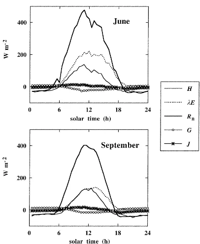
Typical diurnal variation of energy fluxes is shown in Fig. 8. During the daylight hours, the Bowen ratio
β was equal to 0.48 under non-limiting soil water
and maximum LAI (Fig. 8, top). When soil water de-creased (Fig. 8, bottom, September 1997),βincreased to 0.79. Soil heat flux and heat storage in the vege-tation were much lower than latent and sensible heat fluxes: they did not exceed 5% of the net radiation.
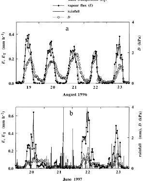
Typical examples of diurnal courses of stand sap flow and of vapour fluxes are shown in Fig. 9a for a bright period and in Fig. 9b for a rainy period. On bright days, during the leafy phase, diurnal pat-terns of stand sap flow and of vapour fluxes were very close, although sap flow showed smoother short term variations than vapour flux. However, for rainy days, much higher vapour fluxes than sap flow were measured (typically 0.6 mm h−1 versus 0.2 mm h−1, respectively). Most of the vapour flux originated in in-tercepted water evaporation, while sap flow remained very low. Comparison of half hourly fluxesEandET
condi-Fig. 6. Sap flux density in beech, Fd, expressed as percentage of maximum value, as a function of tree basal area or tree cir-cumference. Data are standardised as the ratio of actual sap flux density to average sap flux measured in dominant trees (basal area > 7500 mm2).
tions. During dry conditions,ET was linearly related
toE(r2=0.85) with a slope of 0.77. Only a poor
re-lationship (r2=0.46) betweenEandETwas observed for wet conditions. The quite large scatter of data was due to the rapid variation in E measurements, while
ET variation was more buffered, as shown in Fig. 9.
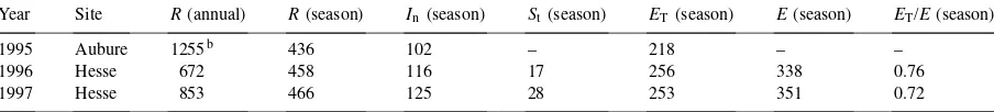
Table 3 gives the cumulated values of rainfall, net interception, transpiration, and of total evapotranspi-ration for the two vegetation periods. Annual stand transpiration and evapotranspiration were very similar for the 2 years. During 1996, the limited tree transpi-ration due to water stress was compensated by higher transpiration rates during the first part of the season, due to higher vapour pressure deficit and air tempera-ture than in 1997.
Table 3
Cumulative values of rainfall (R), net interception (In), stemflow (St), stand transpiration (ET) and total evapotranspiration (E)a Year Site R(annual) R(season) In(season) St (season) ET (season) E(season) ET/E(season)
1995 Aubure 1255b 436 102 – 218 – –
1996 Hesse 672 458 116 17 256 338 0.76
1997 Hesse 853 466 125 28 253 351 0.72
aThe season is defined as lasting from budbreak (2 May) to leaf fall (27thOctober).ETwas computed from scaled sap flow measurements, Ewas measured over the stand by eddy covariance technique.
bData are expressed in mm.
Fig. 7. Variation of 24 h-totals of vapour flux (E) and of stand transpiration (ET) for the 2 years of experiment (1996–1997) in the Hesse beech forest. Also shown (top) is the variation of leaf+stem area index (SAI), calculated from absorbed global radiation by the canopy (see text). Winter SAI represents trunk and branch area indices. Bottom, the seasonal course of gross rainfall,P, and relative extractable water in the soil (θe) obtained from neutron probe and TDR measurements.
3.3. Canopy conductance: modelling and validation
3.3.1. Calibration
Tree and total canopy conductances were derived from climatic data and from either sap flow or eddy co-variance measurements, using the Penman–Monteith equation (see Section 2). In this study, we analysed
Fig. 8. Monthly average diurnal variation of the energy fluxes in the beech stand: net radiation (Rn), sensible flux (H), latent flux (λE), soil heat flux (G) and heat storage in the vegetation (J). Top: high soil water content (June 1997), bottom: low soil water content (September 1997).
Stewart, 1988), which is defined as follows:
gc=gcmax(R, D)f (T )g(θe) (5)
wheregcmax (mm s−1) is the canopy conductance, in
the absence of limitation due to temperature or to soil water deficit, depending on global radiation (W m−2) and on vapour pressure deficitD(kPa),f(T) andg(θe)
are the limiting functions of air temperature and of soil water deficit, respectively.
Maximum tree canopy conductancegcmaxwas
cal-ibrated using measurements performed from 29 May to 18 July 1996 in the Hesse forest. This period cor-responds to the time when: (i) LAI had stabilised to its maximum value (as verified from the variation of radiation intercepted by the canopy), and (ii) soil wa-ter was not limiting (i.e. relative extractable wawa-ter was higher than 0.4).
Only data measured on dry foliage conditions when fitting the gcmax function were used, so periods of
rainfall and the 2 h following rainfall events were eliminated. Using a two variable non-linear
regres-sion (Gauss–Marquart algorithm), equations forgcmax
(6) andgcT (9) were fitted. As there could be a time
lag between canopy transpiration and sap flow, due to non-conservative water fluxes during the day, the fol-lowing calculations were performed. We introduced three increasing time lags of 0.5, 1.0 and 1.5 h to these data, the sap flow lagging behind climatic vari-ables. For each set of time-lagged data, we applied the non-linear regression and compared regression coefficients: r2 was 0.860, 0.768, 0.713 and 0.695 for the increasing time lags from 0 to 1.5 h. As the highest correlation was calculated for zero time lag, we concluded that there was no significant time lag between transpiration and sap flow in beech, at least under high water supply. The absence of time lag was also confirmed by comparing the time courses ofE
andETin Fig. 9.
The relationship relatinggcmax to global radiation
above the stand (R), and to air vapour pressure deficit (D) are shown in Fig. 11. Then, in order to calculate the effects of the other environmental variables, we plotted the ratio of calculated gc to modelled gcmax
against air temperature (Fig. 12a) and against relative extractable water in the soil (Fig. 12b). We observed a strong limitation ofgc for air temperatures below
15–17◦C, and we assumed this decrease to be linear
from 17 to 10◦C (Eq. (7)). With increasing soil water
deficit,gc/gcmax decreased logarithmically (Fig. 12b,
Eq. (8)). We fitted the following functions:
gcmax=
Slightly lower values ofgcmax were found in 1997
Fig. 9. Diurnal variation of vapour flux (eddy covariance),E, and of stand transpiration (scaled from sap flow measurements),ET, during successive days under sunny (a) and rainy (b) conditions in the Hesse forest. Air vapour pressure deficit (D) and rainfall are also shown on the secondY-axis.
Total dry canopy conductancegcTfollowed a
simi-lar relationship toRandD:
gcT=
R
R+550
46.78 1+0.948D
(9)
Higher values forgcTthan forgcwere observed (Fig.
11). The response of gcT to R and D variation was
slightly different than forgc, total conductance
show-ing a less pronounced decrease with increasshow-ingDthan forgc.
For wet foliage, the inverted Penman–Monteith equation was used to estimate ga from the eddy
covariance data. Although there was no evident re-lationship between ga and windspeed, estimated ga
was in the same range (0.1–0.8 m s−1) than values calculated from the Eq. (3).
We calculated the decoupling coefficient omega (Jarvis and McNaughton, 1986), for non-limiting soil water, from the climatic variables and from calcu-latedga andgc. We found a high degree of coupling
Fig. 10. Relationship between vapour flux measured above the beech stand (eddy covariance),E, and scaled-up tree transpiration measured using sap flow technique,ET. Half hourly data of 1996 and 1997. Dry (crosses) and wet (circles) canopy conditions are separated. The two lines indicate the best fits for dry (full line) and wet (dotted line) conditions. Equations are ET=0.771 E (r2=0.85), andET=0.425E(r2=0.46) for dry and wet canopy conditions, respectively.
the variation of omega for dry canopy conditions: the lower the windspeed, the higher the decoupling coefficient was. The strong coupling between canopy and the atmosphere was due to a much higher aero-dynamic conductance compared to the canopy con-ductance (typically 10–50 fold).
Fig. 11. Calculated tree (gc) and total (gcT) canopy conductance for water vapour in 1996 as a function of air vapour pressure deficit (D) and of global radiation (half hourly values), for a period when LAI was at its maximum and when both air temperature and soil water content were not limiting.
3.3.2. Validation: modelling of stand transpiration in the Aubure beech forest
After calibrating Eq. (5) on the Hesse forest data set, modelled canopy conductance was introduced in the Penman–Monteith equation for modelling stand tran-spiration of the beech stand in the Aubure forest. We compared modelled stand transpiration (ETM), using
Eq. (6) and (7) with weather data measured close to the experimental plot, to the sap flow measurements per-formed in the Aubure stand during 1995. Fig. 13 shows the time course of measured and modelled transpira-tion from mid-June to the beginning of August. For the period of 19–29 June, stand sap flow was slightly lower thanETM, probably because young leaves, even
if fully expanded, had not yet reached their physio-logical maturity. On some days (e.g. 3 and 16 July) transpiration was reduced by rain events due to evapo-ration of intercepted water. It is also to be noticed (Fig. 13), that on some nights (e.g. 20 and 21 July), sap flow did not completely stop. This observation was also reported by Köstner et al. (1998a) in a Norway spruce stand, but this author could not conclude either in the existence of night transpiration, or in the trunk refilling during the night. We also found at Aubure the same effect of air temperature as at Hesse, that strongly reduced tree canopy conductance approximately below 15–17◦C.
Over the period between 18 June and 27 August,
Fig. 12. Ratio of actual to maximum tree canopy conductancegc/gcmax (see text) as a function of (a) air temperature (6 June–19 July 1997) and (b) relative extractable water in the soilθefor periods when LAI was at its maximum. From 20 May to 19 September 1996,θe was estimated daily within each week taking into account input (throughfall) and output (stand evapotranspiration) fluxes. From 19 June to 29 September 1997, data points correspond to weekly measurements ofθe.
in the following equation, calculated from data of Fig. 14 :
ETM=1.055ET r2=0.932 (10)
in whichETM andETare expressed in mm h−1.
Fig. 13. Comparison of stand transpiration (ET) in the Aubure beech forest to estimated transpiration (ETM) using the canopy conductance sub-model calibrated in the Hesse forest during spring–summer period.
4. Discussion
4.1. Water balance and soil water content
Fig. 14. Comparison of modelled (Penman–Monteith model, parameterised with the canopy conductance function obtained at Hesse) to measured stand transpiration in the Aubure beech forest from 18 June to 27 August, corresponding to full leaf development. The line corresponds to the linear regression:ETM=1.055ET.
stands: 14–16% in Neal et al. (1993), 20.3% in Biron (1994), 23% in Aussenac and Boulangeat (1980). This is probably due to rainfall conditions (intensity and frequency). Cumulated stand transpiration (ET), inter-ception (In) and vapour fluxes (E) were similar for
1996 and 1997 (Table 3). For both years, total vapour flux as measured above the stand was markedly lower than the sumE+In. The difference amounted to 34
and 27 mm in 1996 and 1997, respectively. This could be attributed to: (i) a loss of vapour fluxes as measured with the eddy covariance technique, or (ii) underesti-mated measurements during rainfall periods, when the sonic anemometer was wet.
During drought, water absorption by roots from the soil seemed to be strongly dependent on the soil physi-cal properties: we observed that a heavily clayey layer reduced root colonisation and therefore reduced wa-ter extraction. When roots could extend below such a layer (as in Zone 1), water absorption was observed in deeper horizons as reported by Bréda et al. (1995) in an oak stand growing on a similar soil type. Neverthe-less, we observed a large spatial heterogeneity in max-imum extractable soil water in the experimental plot: within a distance of ca. 30 m, maximum extractable water in the soil varied between 130 and 185 mm. This
could induce large spatial variations in tree response during severe drought.
4.2. Sap flow
We observed a general pattern of sap flux density relative to the depth below cambium in the beech stems, independent of tree size. This radial profile of sap flux density observed in our study was very sim-ilar to that reported on older beech trees (Köstner et al., 1998b; S. Lang, personal communication). The sap flux velocity profile seems to be related to wood water content: the highestFd rates were observed in
the wettest peripheral wood layers, which are probably less embolised and contain more living cells than older and more internal layers. Ladefoged (1960) reported that beech sapwood could extend from 10 to 20 an-nual rings, corresponding to 20 to 50 mm xylem thick-ness in our trees. In the present study, no well marked heartwood was found in beech.
living tissues during well watered periods. One ex-planation could be that our measurements were per-formed in young trees, having probably less exchange-able water than bigger trees. It seems that the capac-itance phenomenon has been more often observed in coniferous species (Jarvis, 1975, Schulze et al., 1985, Granier and Loustau, 1994, Loustau et al., 1998) than in broad-leaved trees. In temperate oaks, Granier and Bréda (1996) found a 30 min time lag. Since beech and coniferous species like pines are both characterised by a large sapwood thickness in the trunk, the cause of such difference cannot be attributed to the amount of xylem elements, but probably to the intrinsic capaci-tance properties of the tissues.
Among-tree variability in sap flow was linked to crown status. Dominant trees, of which the crowns in-tercept a high proportion of the incident radiation, ex-hibited higher sap flux densities and therefore much higher total sap flow rates than smaller trees. Be-cause of their ground area distribution, the contribution of dominant trees (C1.3> 300 mm) represented about
79% of the stand transpiration.
4.3. Stand transpiration and canopy conductance
Over the 2 years of measurements, a linear rela-tionship was found between stand sap flow and eddy covariance in the Hesse forest, on a hourly as well as on a daily basis. Stand transpiration was equal to 77% of total evapotranspiration when the canopy was dry. The remaining 23% could, at least partly, be due to soil evaporation. Nevertheless, there is a large uncer-tainty in the difference betweenEandETdue to errors
of measurements in both terms. On the one hand, to-tal forest evaporation could be underestimated, as sus-pected when we compared net radiation to the sum of the energy fluxes measured by eddy covariance. The energy balance closure was not met, the difference was 12% ofRn on average. Even if we made an average
frequency correction of about 8%,Ewould still be un-derestimated. On the other hand, scaling tree transpi-ration to the stand level includes two types of errors: (i) The measurement error on the averageFd, due to
the among-tree variability (see Figs. 5 and 6). It must be emphasised that the accuracy in stand transpiration estimates is very sensitive to the weight given to each sampled tree and to the sample size (see Köstner et
al., 1996, 1998b); (ii) The uncertainty in the scaling factor, the stand ground area. Recent forest inventories (data not shown) performed in the surrounding 10 ha, based on 119 local measurements, showed a large spa-tial variation in the tree ground area, with a coefficient of variation of about 0.18.
In the absence of water stress, Bowen ratio ‘β’
equalled 0.48 on average, i.e. latent heat flux was al-most twice the sensible heat flux. When soil water con-tent decreased during summer, as the result of stomata closure,β increased to 1.25.
As observed here, and reported in other field stud-ies, for non-limiting soil water conditions, tree canopy conductance was shown to vary mainly with radiation and with air vapour pressure deficit. A similar relation-ship toRandDwas found for both estimates of canopy conductance, even if under higher evaporative demand estimatedgcTwas greater thangc(E>ET). Under low
evaporation demand (i.e., whenRandDare low), we could not distinguish between gc and gcT, probably
because of the larger relative errors inEandET
mea-surements. The effect of air temperature ongchas been
less studied than the influence of other environmen-tal variables. In beech, we found that air temperature below a threshold of 17◦C played an important role,
while it was not observed in oak trees (Granier and Bréda, 1996). This rapid decrease ingcwhen air
tem-perature fell below 17◦C was confirmed by the
anal-ysis of the variation ofgcTas calculated from vapour
flux data for the first half (spring and early summer) of the leafy period. Overdieck and Forstreuter (1994) also showed on young beech plants a significant increase in transpiration at the leaf scale, when air temperature increased in the range of 15–20◦C. Nevertheless, this
phenomenon was not observed during September and October; then low temperatures did not affectgc nor gcT.
Table 4
Comparison of modelled canopy conductance in the beech stand to the two models of Herbst (1995), under full leaf expansion, sufficient soil water content, and for different combinations of global radiation (R) and air vapour pressure deficit (D)a R(W m−2) D(kPa) % differences % difference
aDifferences in estimates are expressed relative to Herbst model values.
to environmental factors (radiation, vapour pressure deficit, temperature) appeared to be very similar. Fur-thermore, our canopy conductance function matched also closely with that of Herbst (1995), his gc-model
being calibrated from water vapour measurements per-formed on a 100-year old beech forest in Germany. He proposed two sub-models ofgc(see Herbst (1995);
Eqs. (6) and (7), p. 1013), differing in the effect of global radiation (R): Model 1 used a curvilinear func-tion, whereas Model 2 was linearly related toR. The best estimates were obtained with the linear function of R, while we found that a curvilinear function ex-plained better the observed variation. We compared our estimates ofgcto the two models of Herbst using
different combinations ofRandD, as shown in Table 4. The relative difference between Herbst’s and our
gc estimates ranged from 5 to 14%, and from−38%
to 6% when using models 1 and 2, respectively. This would lead to typical differences in stand transpira-tion of less than 10%. Shuttleworth (1989) and Granier et al. (1996a) previously reported such similarities in the diurnal patterns of gc when comparing various
forest ecosystems. However, when comparing canopy conductance in different forest stands, it seems that LAI plays a more important role than species compo-sition (Granier et al., in prep.). Transpiration rates of our two beech stands were comparable, probably be-cause LAI were very similar.
A strong coupling between the beech canopy and the atmosphere was found here: omega factor remained lower than 0.2, as reported elsewhere for a beech forest by Herbst (1995) and for various other for-est stands (Granier and Bréda, 1996, Granier et al., 1996b, c).
5. Conclusions
This work showed that the combination of two methods measuring water vapour fluxes at different spatial scales was possible, however only under some precautions. Nevertheless, we showed that some un-certainties were associated with both methods. Eddy covariance did not give reliable measurements during rainfall, thus rainfall interception could not be mea-sured accurately. For the uncertainties of the energy balance closure, no clear reason was found.
Surprisingly, we did not find significant differences in forest transpiration when comparing beech stands growing under various conditions of age, climate and soil.
Acknowledgements
This work was supported by: (1) the European pro-gramme Euroflux (ENV4-CT95-0078) coordinated by R. Valentini, (2) the French National Forest Service (ONF), 3) a multidisciplinary programme on interac-tions between Man and Environment of CNRS: ‘Envi-ronnement, Vie et Sociétés’). The French government (Ministry of Research) granted a PhD student.
We are also grateful to P. Gross and P. Berbigier for eddy covariance set-up and monitoring, to B. Clerc, F. Willm, Y. Lefèvre and D. Imbert for their valuable technical help in the field, and to Oliver Brendel for commenting on the final version of the article.
References
Aubinet, M., Grelle, A., Ibrom, A., Rannik, Ü., Moncrieff, J., Foken, T., Kowalski, A.S., Martin, P.H., Berbigier, P., Bernhofer, CH., Clement, R., Elbers, J., Granier, A., Grünwald, T., Morgenstern, K., Pilegaard, K., Rebmann, C., Snijders, W., Valentini, R., Vesala, T., 1999. Estimates of the annual net carbon and water exchange of forests: the EUROFLUX methodology. Adv. Ecol. Res. 30, in press.
Aussenac, G., Boulangeat, C., 1980. Interception des précipitations et évapotranspiration réelle dans des peuplements de feuillu (Fagus silvatica L.) et de résineux (Pseudotsuga menziesii (Mirb) Franco). Ann. Sci. For. 37, 91–107.
Black, T.A., 1979. Evapotranspiration from Douglas fir stands exposed to soil water deficits. Water Resources Res. 15, 164– 170.
Bréda, N., Granier, A., Barataud, F., Moyne, C., 1995. Soil water dynamics in an oak stand I. Soil moisture, water potentials and water uptake by roots. Plant soil 172, 17–27.
Gash, J.H.C., Shuttleworth, W.J., Lloyd, C.R., André, J.-C., Goutorbe, J.-P., Gelpe, J., 1989. Micrometeorological measurements in Les Landes forest during HAPEX-MOBILHY. Agric. For. Meteorol. 46, 131–147.
Granier, A., 1985. Une nouvelle méthode pour la mesure du flux de sève brute dans le tronc des arbres. Ann. Sci. For. 42, 193–200. Granier, A., 1987. Evaluation of transpiration in a Douglas-fir stand by means of sap flow measurements. Tree Physiol. 3, 309–320. Granier, A., Bréda, N., 1996. Modelling canopy conductance and stand transpiration of an oak forest from sap flow measurements. Ann. Sci. For. 53, 537–546.
Granier, A., Loustau, D., 1994. Measuring and modelling the transpiration of a maritime pine canopy from sap-flow data. Agric. For. Meteorol. 71, 61–81.
Granier, A., Biron, P., Bréda, N., Pontailler, J.-Y., Saugier, B., 1996a. Transpiration of trees and forest stands: short and long-term monitoring using sapflow methods. Global Change Biol. 2, 265–274.
Granier, A., Biron, P., Köstner, B., Gay, L.W., Najjar, G., 1996b. Comparisons of xylem sap flow and water vapour flux at the stand level and derivation of canopy conductance for Scots pine. Theor. Appl. Climat. 53, 115–122.
Granier, A., Ceschia, E., Damesin, C., Dufrêne, E., Epron D., Gross, P., Lebaube, S., Le Dantec, V., Le Goff, N., Lemoine, D., Lucot, E., Ottorini, J.M., Pontailler, J.Y., Saugier, B., 2000. The carbon balance of a young beech forest. Func. Ecol., (in press).
Granier, A., Huc, R., Barigah, S.T., 1996c. Transpiration of natural rain forest and its dependence on climatic factors. Agric. For. Meteorol. 78, 19–29.
Herbst, M., 1995. Stomatal behaviour in a beech canopy: an analysis of Bowen ratio measurements compared with porometer data. Plant Cell Environ. 18, 1010–1018.
Jarvis, P.G., 1975. Water transfer in plants. In: de Vries, D.A., Afgan, N.G., (Eds.), Heat and Mass Transfer in the Plant Environment. Part 1. Scripta Book Co., Washington D.C., pp. 369–374.
Jarvis, P.G., 1976. The interpretation of the variations in leaf water potential and stomatal conductance found in canopies in the field. Phil. Trans. R. Soc. London 273, 596–610.
Jarvis, P.G., McNaughton, K.G., 1986. Stomatal control of transpiration: scaling up from leaf to region. Advances in Ecological Research. Academic Press, London, 15, pp. 1–49.
Köstner, B., Biron, P., Siegwolf, R., Granier, A., 1996. Estimates of water vapor flux and canopy conductance of Scots pine at the tree level utilizing different xylem sap flow methods. Theor. Appl. Climat. 53, 105–113.
Köstner, B., Falge, E.M., Alsheimer, M., Geyer, R., Tenhunen, J.D., 1998a. Estimating tree canopy water use via sapflow in an old Norway spruce forest and a comparison with simulation-based canopy transpiration estimates. Ann. Sci. For. 55, 125–139. Köstner, B., Granier, A., Cermák, J., 1998b. Sap flow
measurements in forest stands — methods and uncertainties. Ann. Sci. For. 55, 13–27.
Köstner, B.M.M., Schulze, E.D., Kelliher, F.M., Hollinger, D.Y., Byers, J.N., Hunt, J.E., McSeveny, T.M., Meserth, R., Weir, P.L., 1992. Transpiration and canopy conductance in a pristine broad-leaved forest of Nothofagus: an analysis of xylem sap flow and eddy correlation measurements. Oecologia 91, 350– 359.
Ladefoged, K., 1960. A method for measuring the water consumption of larger intact trees. Physiol. Plant. 13, 648–658. Loustau, D., Domec, J.C., Bosc, A., 1998. Interpreting the variation in xylem sap flux density within the trunk of maritime pine (Pinus pinaster Ait.): application of a model for calculating water flows at tree and stand levels. Ann. Sci. For. 55, 29–46. Moncrieff, J.B., Massheder, J.M., de Bruin, H., Elbers, J., Friborg, T., Heusinkveld, B., Kabat, P., Scott, S., Soegaard, H., Verhoef, A., 1997. A system to measure surface fluxes of momentum, sensible heat, water vapour and carbon dioxide. J. Hydrol. 188–189, 589–611.
Neal, C., Robson, A.J., Bhardwaj, C.L., Conway, T., Jeffery, H.A., Neal, M., Ryland, G.P., Smith, C.J., Walls, J., 1993. Relationships between precipitation, stemflow and throughfall for a lowland beech plantation, Black-Wood, Hampshire, Southern England — findings on interception at a forest edge and the effects of storm damage. J. Hydrol. 146, 221–233. Overdieck, D., Forstreuter, M., 1994. Evapotranspiration of beech
stands and transpiration of beech leaves subject to atmospheric CO2 enrichment. Tree Physiol. 14, 997–1003.
Schulze, E.D., Cermak, J., Matyssek, R., Penka, M., Zimmermann, R., Vasicek, F., Gries, W., Kucera, J., 1985. Canopy transpiration and water fluxes in the xylem of the trunk ofLarixandPicea trees: a comparison of xylem flow. Oecologia 66, 475–483. Shuttleworth, W.J., 1989. Micrometeorology of temperate and
tropical forest. Phil. Trans. R. Soc. London B 324, 299–334. Stewart, J.B., 1988. Modelling surface conductance of pine forest.
Agric. For. Meteorol. 43, 19–35.
Tenhunen, J.D., Valentini, R., Köstner, B., Zimmermann, R., Granier, A., 1998. Variation in forest gas exchange at landscape to continental scales. Ann. Sci. For. 1–2, 1–11.