Constrained conjunctive-use for endogenously separable water
markets: managing the Waihole–Waikane aqueduct
Rodney B.W. Smith
a,∗, James Roumasset
b,1aDepartment of Applied Economics, University of Minnesota, Saint Paul, MN 55108-6040, USA bEconomics Department, University of Hawaii, Honolulu, HI 96822, USA
Abstract
An internal solution to an optimal control problem involving conjunctive-use of surface and groundwater may be inapplicable if water is not sufficiently fungible across space and time. We provide a more general solution and apply it to the problem of allocating a limited amount of water from the Ko‘olau mountains to two Oahu water districts separated by those mountains. The solution involves initially allocating all of the mountain water to the district supplied by groundwater but eventually allocating all of the water to the district supplied by surface water. The conditions for an internal solution hold only in the intervening years when some mountain water is allocated to each district. © 2000 Elsevier Science B.V. All rights reserved.
Keywords: Resource economics; Conjunctive-use
1. Introduction
As in many states, water management in Hawaii is organized according to separate water districts. It is commonly assumed that efficient management can be accomplished by managing each district separately and then trading across districts until the value of water is equalized across districts. This view not only glosses over spatial issues such as transport costs and conveyance losses, but also overlooks complications that arise in the context of conjunctive-use. Previous authors have shown how to incorporate transportation costs and water quality into water allocation models such that the marginal benefit at each point in the system is equal to its corresponding full marginal
∗Corresponding author. Tel.:+1-612-625-8136;
fax:+1-612-625-2729.
E-mail addresses: [email protected] (R.B.W. Smith),
[email protected] (J. Roumasset).
1Tel.:+1-808-956-7496; fax:+1-808-956-4347.
cost, including the conveyance costs as well as pollu-tion costs (see, e.g. Chakravorty et al., 1995; Krulce et al., 1997). Similar conditions apply to the problem of interbasin water transfers. Such models, however, require that preconditions guarantee the feasibility of an internal solution. When it is possible to transport the resource from one market to the other, however, one could encounter situations where the amount of water available for transport is insufficient to equate water values across districts, and hence, preempt the possibility of obtaining internal solutions.
In the present paper, we are concerned with a case in which there are limits to allocating water between neighboring markets. For illustrative purposes we consider a situation in Hawaii involving two water districts that share a common source. Because each district has its own source as well as the common source, corner solutions are possible in which all of the common source is allocated to one district or the other. The situation is further complicated by the prob-lem of conjunctive-use; one district relies primarily
on groundwater from the Pearl Harbor Aquifer, while the other relies primarily on surface water. Ordinarily, one would solve for the extraction/allocation profile that simultaneously solves for optimal depletion of the aquifer up to some steady state and optimal spa-tial distribution of the total water available in each time period (Tsur, 1991; Tsur and Graham-Tomasi, 1991). In the present problem, however, one must solve for constrained conjunctive-use, admitting the possibility that water scarcity may become greater in one market than the other — even when it already receives all of the available common water. Since the optimal allocation may be different in each time pe-riod, this involves choosing an allocation vector for the common source as well as an optimal extraction profile for the groundwater aquifer, both of which are interdependent. The model we present is a step in the direction of developing a general spatial/intertemporal model of conjunctive-use water management with multiple water sources and transport technologies.
Section 2 provides a theory of conjunctive-use with limited possibilities of moving water from one district to another. Section 3 illustrates the model for a current conflict between water districts on the Island of Oahu. Some conclusions and policy implications are offered in Section 4.
2. Model
Consider two adjacent water districts divided by a mountain range, with districts 1 and 2 indexed byi=
1,2. Each district contains a fully integrated water market with its own aggregate demand function. An aqueduct system traverses the mountain range and the constant flow of water through the aqueduct can be used to supply either district with water. Denote the daily flow of aqueduct water byS¯ and the amount of aqueduct water diverted to districts 1 and 2 at timet bys1(t )ands2(t ), respectively. The per-unit cost of
gravity driven transport of the water to district i is denotedτ0i ≥0.2
District 1 has access to a coastal aquifer, where the amount of aquifer water extracted at timet is denoted
2Each district’s transportation cost may be thought of as
the mean cost to that district. For methods of incorporat-ing intra-district transport cost differences, see Chakravorty and Roumasset (1991) and Chakravorty et al. (1995).
as q(t ). We follow Krulce et al. (1997) in modeling aquifer characteristics. Leth(t )denote the head of the aquifer above sea level at timet, and letl(h)denote the amount of water leaking from the aquifer given head levelh. The higher the head level, the larger the sur-face area from which water can leak, and the greater the water pressure on the existing surface area; sug-gesting that leakage increases in head. We assume that the leakage function satisfies the following properties: l(h) ≥ 0, l′(h) > 0, l′′(h) ≥ 0, andl(0) = 0, i.e., leakage is a positive, increasing, convex function of head. Aquifer inflow (from rainwater) occurs at rate w. Unexploited, the aquifer head rises to the levelh¯ where leakage exactly equals inflow,w=l(h)¯ . Since leakage increases as head levels increases and head levels fall as the aquifer is exploited, it follows that w−l(h)≥0. The aquifer head evolves over time ac-cording toh(t )˙ =w−l(h(t ))−q(t ).3 The average cost of extracting water from the aquifer isc(h)≥0, wherec′(h) <0,c′′(h)≥0, and limh→0c(h)= ∞.
In addition to aqueduct water, district 2 receives a daily flow of surface water and sustainable ground-water yields denoted SF. Both districts have access to exotic backstop technologies, e.g., desalination. Letb1(t )andb2(t )denote the timet amount of the
backstop resource supplied to districts 1 and 2, respec-tively, and represent the per-unit cost of the backstop technology (desalination) byp¯. The per-unit cost of transporting aquifer or backstop water to end users in district 1 is denoted asτ1≥0, while the per-unit cost
of transporting surface or backstop water to end users in district 2 is denoted asτ2≥0.
GivenSF and access to the backstop technologies, a water commission is responsible for managing aque-duct allocation and water extraction rates from the aquifer. The timet water demands for districts 1 and 2 are represented by D1(p1(t ), t ) and D2(p2(t ), t ),
respectively. Herepi(t )is the timet price of water in
districti. Fori=1,2 and for allt, we assumeD1i = ∂Di/∂pi < 0 and Di2 = ∂Di/∂t ≥ 0: demand
is strictly decreasing in price and demand is non-decreasing over time. Denote the time t inverse demands for district i by Ni(xti, t ), where xti is the time t quantity of water demanded in dis-trict i. Given the properties of Di, it follows that N1i = ∂Ni/∂xti < 0 and N2i = ∂Ni/∂t ≥ 0,
i = 1,2. The gross surplus of water in district i is given byRNi(x, t )dx. Then the water commission’s problem can be represented as choosing the trajectory
{q(t ), b1(t ), s1(t ), b2(t ), s2(t )}t∈(0,∞), to maximize:
ditional unit of aqueduct water to districti. Suppress-ingt, the necessary conditions for an optimal solution are
and the complementary slackness conditions:
∂H
et al. (1997), we assume the cost of desalination is high enough so that water is always extracted from the aquifer and (2.4) always holds with equality,
λ=p1−c(h)−τ1. (2.9)
By Eq. (2.9), the in situ shadow price of district 1 water,λ, is equal to the market price of water in district 1 less extraction and transport costs. Also, rearranging Eq. (2.3) gives
The left-hand side of (2.10) is the marginal benefit of extracting water today. The right-hand side is the marginal user cost, i.e. the lost present value of extract-ing water. The first right-hand side term is the fore-gone present value from not appropriating the capital gain associated with saving the marginal unit of water. The second term is the present value lost from having to incur higher extraction costs in the future. The third term is the (partially offsetting) reduction in marginal user cost due to the higher recharge associated with the lower head level. Alternatively, expression (2.10) can be rewritten as
λ= ˙
λ−c′(h)q r+l′(h) ,
Eqs. (2.5) and (2.7) describe what happens to market price when the backstop technology is adopted. These equations can be rewritten as
pi−τi ≤ ¯p, i=1,2. (2.11)
If the shadow price of water in districtiis less than the cost of desalination, then desalination does not occur on that side. When either district uses desalination, the price of water on that side must be equal to the per-unit cost of desalination, i.e., pi −τi = ¯p. Hence with
desalination,pi−τi = ¯pimplies that expression (2.3)
can be written asλ= ¯p−c(h); the in situ shadow price of water varies only with average extraction costs, i.e.,
˙
λ= −c′(h)h˙. Next, combineλ= ¯p−c(h)−τ1and ˙
λ = c′(h)h˙ with Eqs. (2.2) and (2.3), and eliminate λ,λ,˙ andh˙. Using this we see that when desalination is adopted in district 1,
¯
p−c(h)= −[w−l(h)]c
′(h)
r+l′(h) >0. (2.12)
Recall from (2.9) that the left-hand side of Eq. (2.12) is the in situ shadow price of water, i.e. the marginal benefit of extracting water in the optimal program. The right-hand side is the marginal user cost once the aquifer reaches a steady state. Note that unlike the case of non-renewable resources, the scarcity rent,λ, does not go to zero when the backstop is employed. As shown in the application, the steady state scarcity rent can, in fact, be several times larger than the extraction cost.
Krulce et al. (1997) argue that the optimal head level satisfying (2.3) is unique and when desalination is used the optimal head level is maintained at a constant level, denoted h∗. In such a case, extraction rates must be equal to the net inflow of water to the aquifer and extraction rates are constant, denoted asq∗.
2.1. Aqueduct management
The optimal allocation of aqueduct water is gov-erned by Eq. (2.6) and must satisfy the following conditions:
p1(t )−τ1=p2(t )−τ2, γ1(t )=γ2(t )=0, p1(t )−τ1> p2(t )−τ2, γ1(t )=0, γ2(t ) >0, p1(t )−τ1< p2(t )−τ2, γ1(t ) >0, γ2(t )=0.
If the equilibrium price paths are moving together then both sides are receiving aqueduct water. If over a pe-riod of time equilibrium prices are such thatp1(t )− τ1 < p2(t )−τ2, then at some earlier point in time
district 2 received (and continues to receive) all of the aqueduct water (s1t = 0). If, instead p1(t )−τ1 > p2(t )−τ2, then at some earlier point in time district
1 received all of the aqueduct water(s1= ¯S). As one
might imagine, the higher the transport cost is for one district relative to the other, the less aqueduct water the relatively higher transport cost district will receive. When prices have diverged the allocation rule is simple: divert all of the aqueduct water to the side with the highest price. However, when prices are moving together and the backstop technology has not been adopted, the allocation rule is a bit more complex. To see hows1 behaves in such a case, take the time
derivative of the equilibrium relationship (2.6):
d
Given that prices are moving together it follows that (d/dt )(∂H /∂s1)=0. Also, since the backstop
tech-nology has not been reached:b˙1= ˙b2=0. Then, N21+(q˙+ ˙s1)N11=N22− ˙s1N12. (2.14)
Price movements in each market are the result of two effects. Holding water consumption constant, the time effectN2i is the change in price induced by a shift in districtidemand at timet. The direct demand effects (q˙ + ˙s1)N11 and −˙s1N12 are the respective price
re-sponses in districts 1 and 2 to changes in consumption levels at time t. For either market, if the time ef-fect dominates the direct demand efef-fects, then prices increase. Otherwise, prices remain constant or fall.
In equilibrium, the quantity demanded must equal quantity supplied, orq+s1=D1(p1, t ). Taking the
time derivative of this equilibrium condition givesq˙+ ˙
s1 = D11p˙1+D21. Substituting this time derivative
into expression (2.14) and rearranging terms gives the desired behavior ofs1:
˙ s1=
N22−[N21+(D11p˙1+D21)N11]
Given that N12 < 0, if the second district’s shift in demand is large (small) enough relative to the total changes in the other district’s demand, then the amount of aqueduct water diverted to district 2 should be in-creased (dein-creased). There are potentially many pat-terns of optimal aqueduct water diversion schemes. For example, if prices are increasing and demand in district 2 is always increasing more quickly over time than demand in district 1, then more and more aque-duct water will be shifted to district 2. However, even if prices are increasing and demand in district 1 is shift-ing more rapidly than that in district 2, it is unclear whether district 1 should receive an increasing share of aqueduct water. For instance, if the first district’s direct demand effects are large enough relative to its time effects, then it is possible for the time shifts in the second district to dominate the first district’s net demand effects. In such a case the first district would receive increasing quantities of aqueduct water.
If prices move together and reach the backstop at the same time, then the amount of water to divert to
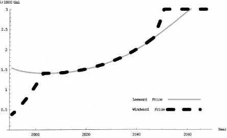
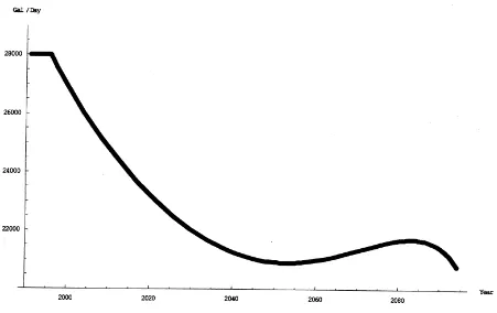
Fig. 1. Optimal price trajectories wheng1=2%,g2=1.5%.
either side is arbitrary — the desalination costs saved by the aqueduct water is the same regardless of its allocation. If backstop technology costs were higher on one side than the other, however, then the water manager is not indifferent about where the aqueduct water is sent. One would expect that if desalination were higher in district 2 than district 1, then if district 1 reached the backstop technology first then district 1 could possibly receive all of the aqueduct water. Then after the price in district 2 reached the backstop price in district 1, district 2 would eventually receive all of the aqueduct water and keep it even after reaching the backstop technology.
2.2. The optimal price and quantity trajectories
The choice ofq, s1, b1andb2must satisfy several
conditions simultaneously. To facilitate the algorithm design we observe that Eq. (2.6) can be used to define s1in terms ofq, b1, andb2. The relationship between
response function:
s1∗(q, b1, b2)=arg min s1
{|N1(q+b1+s1,·)−τ01 −[N2(SF +b2+ ¯S−s1,·)+τ02]|}
subject to s1∈[0,S¯], q, b1, b2≥0,
(2.16)
where the aqueduct response function gives the opti-mal rate at which aqueduct water should be diverted to district 1, given desalination and aquifer extraction rates. Introducing the aqueduct response function into the optimal control problem is accomplished by not-ing that, in equilibrium, water supply in district 1 must be equal to its quantity demanded, i.e.,q+b1+s1∗= D1(p
1,·), or
q =D1(p1,·)−b1−s1∗(q, b1, b2). (2.17)
Then, letq∗denote the (possibly implicit) solution to (2.17), and substituteq∗into (2.2). Finally, combining λ=p1−c(h)−τ1andλ˙ = ˙p1−c′(h)h˙with Eqs. (2.2)
and (2.3) (and eliminatingλ,λ˙, andh˙) yields the
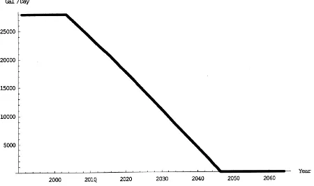
fol-Fig. 2. Optimal allocation of tunnel water to the Leeward market wheng1=2%,g2=1.5%. lowing system of differential equations:
˙
h(t )=w−l(h(t ))−q∗(t ), (2.18)
˙
p1(t )=[r+l′(h(t ))][p1(t )−c(h(t ))−τ1]
+[w−l(h(t ))c′(h(t )). (2.19)
Eq. (2.18) describes the optimal trajectory of the aquifer head and Eq. (2.19) is the optimal trajectory of district 1 water price. The optimal trajectory ofs1∗ is recovered usingq∗, and the optimal trajectory of district 2 water price is recovered by substitutings1∗ into that district’s inverse demand curve.
earlier point in time that district would have received all of the aqueduct water. For example, say the relative acceleration of water demand is higher in the second district. In such a case, in order to equate prices across markets the second district would receive more and more aqueduct water. Eventually, the second district would get all of the aqueduct water, after which the second district’s price would begin rising more rapidly than water prices in the first district. Once the price in district 2 reached backstop levels, desalination would begin on that side. As for the price in district 1, it would eventually either reach backstop levels or level off at some level below district 2 levels (possibly even fall). Several alternative scenarios are examined in the following section based on a situation in Oahu in the State of Hawaii.
3. Application: optimal water management on Oahu
To illustrate an application of the above principles, we reconsider the water management problem
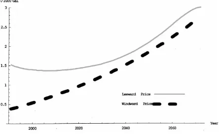
inves-Fig. 3. Optimal price trajectories wheng1=2% andg2=0.4%.
tigated by Moncur et al. (1998), where the relative merits of diverting a constant amount of surface water to each side was investigated. However, as the authors suggested, the optimal allocation of aqueduct water would likely vary over time. A numerical analysis of the interbasin transfer problem requires specification of the leakage functionl(h), the extraction cost func-tion c(h), and the inverse demand functions for the leeward side (district 1) and the windward side (dis-trict 2),N1(·,·)andN2(·,·).
Using the hydrological studies of Mink (1980), the leakage function estimated by Krulce et al. (1997) is l(h)=0.2497h2+0.022h, wherel(h)is measured in mgd (million gallons per day) andh∈(0,33.5). The extraction cost function used in Krulce et al. (1997) is c(h) = c0(h0/ h)n, where c0 = $ 0.283 is initial
extraction costs in 1991,h0=15 is the initial head in
1991, andn=2 is the rate at which extraction costs approach infinity (see Moncur and Pollock, 1988).
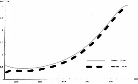
Fig. 4. Optimal price trajectories wheng1=1.4% andg2=0.5%.
will grow over the foreseeable future, while leeward agricultural water demand is expected to fall. Accord-ingly, we decompose leeward demand into residential and agricultural demand. We assume windward ur-ban and agricultural demand will grow at the same rate. We represent leeward demand by D1(p1t, t )= α11eg11t(p1t+cD1)
−η+α
12eg12t(p1t+cD1)
−η, where α11eg11t(p1t + cD1)
−η is leeward urban demand.
Windward demand is represented by D2(p2t, t ) = α2eg2t(p2t +cD2)
−η from i = 1,2. Here p
it is the
timet wholesale price of water in market i, cDi the
distribution cost (net transport costs) in district i, η the elasticity of demand, g11, g12, and g2 are the
growth rates of leeward urban, leeward agricultural, and windward demand, respectively. The parameters α11 and α12 normalize leeward urban and
agricul-tural demand to actual 1991 price and quantity data, while α2 normalizes windward demand.
Follow-ing Moncur et al. (1998), we set cDi = 0.597 and
η = 0.3, and calibrateα11 = 93.63,α12 = 107.47,
and α2 = 40.43 (see Krulce et al., 1997, p. 1223).
Per-unit transport costs are assumed to be given by
τ1 =0.25 and τ2 = 0.45. To derive α2 we observe
that 1991 windward water demand is 38 mgd, imply-ingα2 =38×1.230.3 = 40.43. Finally, we assume SF =38 000 mgd,S¯ =28 000 mgd,p¯ =34 and the real interest rateris equal to 3% (see Roumasset et al., 1983). Relatively straightforward manipulations yield
p1t=N1(q+b1+s1, t ) =
93.63 eg11t+107.47 eg12t
q+b1+s1
(1/0.3)
−0.847,
p2t=N2(SF + ¯S+b2−s1, t ) =
40.43 eg2t
SF + ¯S+b 2−s1
(1/0.3)
−1.047.
In the following analysis we consider three scenarios. In two of the scenarios leeward demand grows at 2% each year, and windward demand grows at either 1.5
4 See Leitner (1992), while Leitner’s estimate is in $ 1984 and
or 0.4% each year. In the last scenario leeward de-mand grows at 1.4% and windward dede-mand grows at 0.5% each year. In each scenario leeward agriculture is assumed to grow at−1%.
In the first scenario urban water demand on the leeward side grows at 2% while windward demand grows at 1.5%. The price and aqueduct water manage-ment trajectories corresponding to this scenario are presented in Figs. 1 and 2. In Fig. 1, the optimal price trajectory for the windward side is given by the dashed curve, while the optimal price trajectory for the lee-ward side is given by the heavy, shaded curve. Note that the leeward price lies above the windward price until a little after 2002, after which the prices move together until a little after 2047. Then the windward price increases more rapidly than the leeward price, hitting the backstop technology about 2 or 3 years later. Fig. 2 shows that the optimal aqueduct water diversion pattern corresponds with what one might expect. In the first few years the leeward side gets all of the aque-duct water. However, a little after 2002 the windward
Fig. 5. Reswitching in optimal sharing rules wheng1=1.4%,g2=0.5%.
side begins receiving some of the aqueduct water, and continues to receive increasing amounts, until in about 2047, it gets all available aqueduct water. This happens because the leeward side can meet increased demand needs by drawing more and more water out of its coastal aquifer, while the windward side faces a relatively fixed source of supply, and hence in order to meet future increased water demand, must resort to the aqueduct water. Without the benefit of the aqueduct source, the value of water would correspondingly rise more rapidly on the windward side. Accordingly, the windward side commands an increasingly larger share of the aqueduct water in order to keep the marginal value of aqueduct water equal across districts. The equality breaks down after the corner solution is reached with all water going to the windward side.
Correspondingly, the windward side never receives any aqueduct water.
Finally, Figs. 4 and 5 correspond to the case where urban leeward demand grows at 1.4% each year while windward demand grows at 0.5% each year. This ex-ample is presented to show that monotonic diversion patterns are not necessarily the rule. In Fig. 4 the op-timal price trajectory on the leeward side is the heavy, shaded curve, while the optimal price trajectory for the windward side is the dashed curve. From 1991 until about 1997 leeward prices are higher than windward prices. After which the price trajectories are identi-cal and both prices reach the backstop technology in 2095. In Fig. 5, we see that it is optimal to allocate the leeward side all of the aqueduct water until about 1997. Then the windward side should begin receiving a monotonically increasingly share of the tunnel water until about 2052, after which the windward allocation should monotonically decrease until 2083. Finally, the windward side should again receive increasing shares of the tunnel water until the backstop technology is reached in 2095.
As with the analytical results presented in Section 2, the illustrative exercises presented here suggest that the optimal extraction vector and aqueduct sharing rules are interdependent and, hence the need to coor-dinate aquifer extraction rates and aqueduct sharing rules. Failure to do so will inevitably lead to ineffi-cient water allocations. As a final note, observe that as-signing water rights and allowing water trading would tend to ameliorate inefficiencies, but even aside from externalities, full efficiency would require that future markets exist for several decades into the future.
4. Conclusion
The model presented here is a step in the direction of developing a general spatial/intertemporal model of conjunctive-use water management with multiple wa-ter sources and transport technologies. The usual as-sumptions that water sources are at a single location or that transport possibilities are characterizable by a matrix of transport coefficients (linear transportation costs) are highly restrictive and typically misrepresent interbasin transfer possibilities. The procedure we out-line requires solving simultaneously for production at each source and time, and consumption in each
dis-trict in each time period. The method can be gene-ralized further to distinguish different locations within districts and to determine flow rates in each part of the conveyance system at each time.
The model focuses on two water districts, each with their own sources, but with each having potential ac-cess to a common, albeit limited, source. The optimal solution involves allocating each successive unit of common water to the district with the highest marginal water value. If water is sufficient, this will lead to equalization of marginal values across districts. If not, the entire amount of water will be allocated to one district or the other, and the efficiency of prices will diverge across districts. In general, it is not possible to determine a priori whether the districts will be in-tegrated in the sense of having the same efficiency prices or will be analytically separate.
If both districts rely on surface water, then optimal allocation of each district can be solved separately in each period and the common water allocated as described above in each period. This method is not available if one or both of the districts relies in part on groundwater. In that case, the periods are interde-pendent. One must solve simultaneously for the op-timal path of groundwater extraction and the opop-timal allocation path of the common water.
The Hawaii application provides a number of lessons that may be of general interest. To the extent that groundwater is underpriced to a greater extent than surface water, as in the two Oahu districts, then the groundwater district should receive initial pri-ority in allocating water from the common source. However, this assumes that the water authorities will simultaneously adopt efficiency pricing or some other mechanism for efficient water allocation. There is no point in allocating more water to the district where water is scarce if that district will continue to waste it.
until some future date. Without such facilities, de-mand growth will eventually cause scarcity in the surface-water district to overtake that of the ground-water district, and priority for common-ground-water alloca-tion will switch from the groundwater district to the surface-water district, as in the Hawaii case.
A third lesson, derivative of the first two, is that re-liable benefit-cost studies of investments in new wa-ter facilities (e.g., pumping stations, dams, aqueducts, tanks, and conveyance structures) cannot be performed without discovering the time-dependent scarcity value of water, thus requiring analogous simulations to those reported here.
The theory and the illustrative exercises underscore the inevitable inefficiency of attempting to manage two such water districts independently. One cannot, as in the Hawaii case, e.g., choose some initial allocation of the shared source and then attempt to adjust the alloca-tion over time according to criteria of relative scarcity in the two districts. The initial allocation itself effects the dynamic path of efficiency of prices, and relative scarcity changes over time. Water trading between the two districts would tend to ameliorate inefficien-cies, but even aside from externalities, full efficiency would require future markets for several decades ahead.
The algorithm discussed in Section 3 renders the in-tertemporal optimal apportionment problem tractable. Other extensions that would improve the normative value of the model for generating recommendations
about optimal management within and across districts include explicit recognition of differential conveyance costs as well as instream benefits and other external effects.
References
Chakravorty, U., Hochman, E., Zilberman, D., 1995. A spatial mo-del of water conveyance. J. Environ. Econ. Mgmt. 28, 25–41. Chakravorty, U., Roumasset, J., 1991. Efficient spatial allocation
of irrigation water. Am. J. Agric. Econ. 73, 165–173. Krulce, D., Roumasset, J., Watson, T., 1997. Optimal management
of a renewable and replaceable resource: the case of coastal groundwater. Am. J. Agric. Econ. 79, 1218–1228.
Leitner, G.F., 1992. Water desalination: what are today’s costs. Desalination and Water Reuse 2, 39–43.
Mink, J., 1980. State of the Groundwater Resources of Southern Oahu. Board of Water Supply, Honolulu, HI.
Moncur, J.E.T., Pollock, R.T., 1988. Scarcity rents for water: a valuation and pricing model. Land Econ. 64, 62–72. Moncur, J.E.T., Roumasset, J., Smith, R., 1998. Optimal allocation
of ground and surface water in Oahu: water wars in paradise. In: Just, R., Netanyahu, S. (Eds.), Conflict and Cooperation on Trans-boundary Water Resources. Kluwer Academic Publishers, Boston.