AUTOMATIC TREE-CROWN DETECTION IN CHALLENGING SCENARIOS
Dimitri Bulatov, Isabell Wayand, Hendrik Schilling
Fraunhofer IOSB, Department Scene Analysis, Gutleuthausstr., 1, 76265, Ettlingen, Germany {dimitri.bulatov, isabell.wayand, hendrik.schilling}@iosb.fraunhofer.de
Commission III, WG III/4
KEY WORDS:3D-modeling, Classification, Hotspots detection, Surface reconstruction, Tree, Watershed Transformation
ABSTRACT:
In this paper, a new procedure for individual tree detection and modeling is presented. The input of this procedure consists of a normal-ized digital surface model NDSM, and a possibly error-prone classification result. The procedure is modular so that the functionality, the advantages and the disadvantages for every single module will be explained. The most important technical contributions of the paper are: Employing watershed transformation combined with classification results, applying hotspots detectors for identifying tree-tops in groups of trees, and correcting NDSM by detecting and geometric reconstruction of small anomalies, such as earth walls. Two minor contributions are made up by a detailed literature research on available methods for individual tree detection and estimation of tree-crowns for clearly identified trees in order to reduce arbitrariness by assigning trees to one of the few types in the output model.
1. INTRODUCTION
There are many applications for 3D models of urban terrain, such as urban planning, navigation, civil security, and others. This is why scientific communities from all over the world pursue more accurate, more precise, and more semantic reconstruction of urban terrain model instances from sensor data. Here, context-based, semantic models mean that the most common instances of urban terrain, such as building, trees, roads, etc., are first de-tected and then reconstructed using soft constraints that charac-terize these instances. Examples of such constraints are piecewise planar building roofs or smooth course of roads. The contribution of this work is to establish a similar workflow for trees. As input we have an ALS (airborne laser scanning) data sampled into an elevation map (denoted also as Digital Surface Model, DSM) and an orthophoto. Starting from a possibly imprecise precise classi-fication result for the tree class, we make use of a soft constraint that a local maximum in a smoothed DSM restricted to the tree class basically corresponds to a tree top. Doing so, we will not only be able to perform individual detection of trees and obtain more information on their position, height and diameter, but also to detect and to correct the systematic errors in the classification result whereas possible.
Detecting and exact modeling trees is important because of many application in forestry, life sciences, but also in security-related issues However, to create a separate model for every tree is com-putationally expensive, especially if interaction is required. In addition, we are striving for a fast procedure in which collection of training data and/or non-local optimization of complicated en-ergy functions are not desirable. As a consequence, we opt for a compromise: after performing single tree detection, we estimate its position, height, and diameter. Then the tree is modeled as a circular or elliptic region. This is sufficient for many applica-tions. Finally, we wish to assign it into one of very few types. For each of these types, a library entry can be created, option-ally adjusted according the the season and day-time, and, finoption-ally, copy-and-pasted within the model on the relevant positions with corresponding scales. This goes hand in hand with the state-of-the-art activities on the semantic representation of urban terrain (Bulatov et al., 2014) in which the resulting models are usually 1) visually appealing, 2) well-compressed, because firstly building
roofs and other planar objects can be represented by a few poly-gons and secondly, because less important objects, such a grass, can be modeled by a few so-called geo-typical objects (dande-lions, blades of grass of difference heights, etc.), 3) easy to mod-ify and 4) inter-operable in the sense that atree modelcan be given further important properties, such as collision geometry, flammability, and many others.
As for the second question, namely, correcting systematic errors, it is well-known that classification in aerial data is often a chal-lenging task because overlapping of classes is always given, espe-cially in the case of trees that occlude other objects: roads, cars, and even buildings. Besides, the particular interest of this paper is dedicated to types of objects that are not included in the list of classes because their appearance is seldom. An example of such ananomalyis an earth hill. If it is grass- or shrubbery covered, it is extremely difficult to differentiate it from a group of trees. Al-ternatively, if such a hill is covered with trees, computation of 3D positions of these tree trunks becomes a very critical issue with respect to the task we set in the last paragraph. Hence, it will be necessary to recognize the anomalies in the terrain and to correct them.
The paper is organized as follows: In Sec. 2 and 3, respectively, we refer to the related work on tree detection and explain the im-portant preliminaries on obtaining tree areas from sensor data. In Sec. 4, four main tools used for individual tree detection are presented while in Sec. 5 we explain how the anomalies in the terrain can be detected and corrected. In Sec. 6, we describe a simple routine for tree crown classification. Then, Sec. 7 sum-marizes the proposed algorithm. The results for a challenging dataset are shown in Sec. 8 while for main conclusions and ideas of future work we refer to Sec. 9.
2. OVERVIEW OF PREVIOUS WORK
is a typical top-down method. Because of many parameters, it is rather unhandy for big data. A sequence of top-hat operators (Andersen et al., 2001) is applied to extract elevated objects of a predefined size. The hill-climbing method due to (Persson, 2001) starts from the classification result. All pixels with height values over a threshold, which lie in the vegetation mask of a strongly smoothed elevation map, are considered as starting points for a local maximum search by moving into the direction of the steep-est gradient.
The contribution of (Pouliot et al., 2002) is a transect approach from the local maximum of the elevation map to the supposed border of tree. Region-growing approach is proposed by (Dalponte et al., 2014) and (Secord and Zakhor, 2007), where features are calculated from the laser and image data and the weights are de-termined by a learning procedure. The work of (Straub, 2003) mentions watershed transformation of the DSM. Edges detected in the images are used to specify borders of hypotheses for the individual tree regions. To assess a hypothesis, he considers geo-metric (area, eccentricity, and second derivative) and radiogeo-metric properties (near-infrared, texture measures, etc.). The conclusion is drawn that combining borders of the watershed regions with edges is only necessary to separate trees and groups of trees from the background, not from each other. In addition, it is a cum-bersome process of edge filtering since some edges are usually within tree crown. Hence, this step is not necessary if we have a reliable classification result; however, it does bring essential improvements in the areas where the classification result is not correct for one of the reason pointed out in the introduction sec-tion. Also, we see that because of its simplicity and efficiency, many other authors use watershed transformation (Wang et al., 2004, Koch et al., 2006, Reitberger, 2010).
3. PRELIMINARIES ON CLASSIFICATION AND EXTRACTION OF TREE REGIONS
The input of our algorithm consists of a DSM and a digital or-thophoto. In what follows, a short description of our method on extraction of tree regions is given. This is important to understand the origin of systematic errors in the classification result.
First, the Digital Terrain Model (DTM) is computed by means of the procedure described in Sec. 2.1 of (Bulatov et al., 2014). By computing the difference between DTM and DSM, we obtain the normalized DSM (NDSM) with clearly distinguished smaller el-evated objects: Buildings, trees, fences, street lamps, earth walls, and others. We perform the classification of the terrain similarly to (Lafarge and Mallet, 2012). Four measures (relative elevation measure fh, planarity measure fp, normalized difference
vege-tation index (NDVI) measure fn, and entropy measure feof the
orthophoto) are computed for each pixelxto distinguish between four main classesl∈{building, tree, grass and ground}. These four measures are collected into energy data terms for the four classes, as described below. A smoothness term penalizing dif-ferences of labels between neighboring pixels is added to the en-ergy function. This function is minimized using the semi-global method of (Hirschmüller, 2008). The resulting label map is post-processed by the median filter and particularly for the classtree, by morphological operations (3×3 or 5×5 closing and opening).
For example, we show here how the data term is built for trees: They are characterized by a non-negligible elevation, by a rather low planarity, a high measure of NDVI, and a high local texture variation, that is, the entropy. Thus, the data termEl(x)=tree for a pixelxto belong to a tree is given by:
El(x)=tree= (1−fh)fp(1−fn)(1−fe), (1)
wheref◦=f◦(x). However, for fwe use a sigmoid-like function asymptotically approaching 0 and 1:
f◦(x) = w(x)
w(x) +1,w(x) =exp
◦(x)−σ κ
(2)
with empirical parametersσandκas well as◦={h,p,n,e}, in-stead of a truncated linear function chosen by (Lafarge and Mal-let, 2012). The reason is that otherwise an elevated region where the term(1−fh)vanishes would become completely a tree or a
building independently on other measures.
4. TOOLS FOR INDIVIDUAL TREE DETECTION
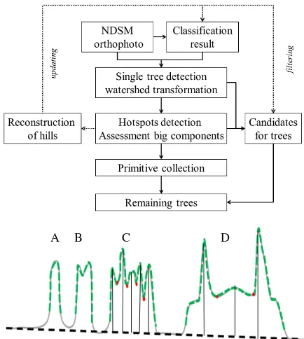
In this section, we describe the four important tools for detection of isolated trees. One can ask why we apply on our data not less than four modules. The reason is that we wish to process large, mostly "smooth and trouble-free" parts of the data by fast, straight-forward modules. Then we basically put these parts of data aside. At the same time, there are anomalies in the data which must be detected and corrected by advanced methods. We show in Fig. 1, top the flow-chart of the proposed algorithm and give more details of it in Sec. 7.
A B C D
Figure 1: Top: overview of the algorithm with dotted lines de-picting correction of the anomalies. Bottom: Proof of principle for individual tree detection with watershed. The height profile for DSM and DTM are shown by solid grey curve and dashed black curve, respectively. The result of classification is depicted by a thick solid green line while centers and borders of different watershed components are shown by vertical black lines and red points, respectively.
bottom, we see that applying
S
in the scenario A leads to a cor-rect detection of tree (which is also the most frequent case). In the scenario B, it is not immediately clear from the DSM alone whether we have two trees pretty near to each other or a single tree with two crowns.Our default method is thewatershedtransformation (
W
) applied on the negative NDSM, but restricted to the classtreeof our clas-sification result. A watershed component has its root in a local minimum of an image and it ends at the shedding line to the neighbored component. As mentioned before, the transforma-tion is very fast and it is suitable to separate trees from each other while the separation from the background has already taken place by means of the classification. However, there are two disadvan-tages of this strategy which either leads to single tree decompo-sitions or to regions that are too big for a single tree. First,W
is sensitive to noise and hence, superfluous components are formed around each local minimum of the input image. This is why we need to perform a median filtering and/or a discretization. As a consequence, the difference of heights between two crowns may get over-smoothed and we get components of a larger size than a usual tree. The other problem stems from classification errors: In the dataset analyzed in Sec. 8, several earth hills not covered with grass usually belong to the tree class and, by applying watershed transformation, we obtain one or more rather big components. This is visualized in Fig. 1: situations B and C show a successful while situation D shows an unsuccessful delineation.In order to bound a component and thus to find an extension of the tree inxandydirection, (Straub, 2003) proposed combina-tion of watershed components and edges in the images. However, the algorithm for Image Segmentation by Optimization of Levels (ISOL) due to (Anderer et al., 1989) has proved to be a suitable alternative. ISOL searches for salient regions, that is, those for which the pixel list does not change significantly after a slightly increasing or decreasing the threshold for gray values. Thus, it is the precursor of the well-known MSER (Maximum Stable Ex-tremal Region) algorithm (Matas et al., 2002), which has pro-duced worse regions. The procedure for detection ofhotspots based on ISOL and denoted here as
H
allows distinguishing trees atop of the hills in scenario D of Fig. 1. In fact, we would ob-tain three nested components: Two for trees and one for the hill, which can be immediately filtered out because of its magnitude. However, because of the nested components, ISOL without post-processing should be rather taken for identifying groups of trees (to be able to model hills) rather than for detection of individ-ual trees. For this latter task, we need a post-processing step in which the components are analyzed by the variance of elevations, by eccentricity and by registering their overlap with other com-ponents (which is time-consuming). Besides computing time, the necessity of forming a discrete image must be mentioned as a disadvantage of ISOL method.After performing extraction of single trees, there can still be com-ponents which are too big and/or too stretched for a single tree. Here, groups of trees are extracted by the procedure
P
(primitive collection) proposed in (Bulatov et al., 2014): The highest tree point yields the position of the first tree. Then, all pixels within a circular region around this point are excluded from the compo-nent; the radius of the circular region corresponds to the typical tree radius of 6m. This procedure is repeated until there are no remaining pixels in the component.5. CORRECTION OF NDSM BY DETECTING AND RECONSTRUCTING HILLS
In this section, we want to find out whether the large components obtained after applying
W
on the NDSM intersected with the treeclass may originate from filtering/discretization artifacts or from anomalies in the DTM/classification. In the latter case, we will perform the reconstruction of the hill surface.
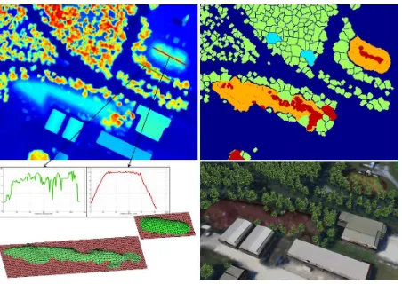
The choice for watershed is made for reasons of speed: We are aware that if the density of trees atop of a hill is very high, it would collapse into very many small regions (hence, ISOL ap-plied on thewholeNDSM) would be more suitable); however, in our dataset earth walls mostly serve exercise purposes and do not contain too many trees. The situation is thus similar to that exem-plified in scenario D of Fig. 1, where a component to be analyzed is formed as a union of three big components with local maxima on the trees and hill top. Cleaning such components from trees – which now are outliers and should be excluded from surface reconstruction – by ISOL and morphological operations (see the red points in Fig. 2, top right), comprise the first step of compo-nent analysis.
Next, for all components, we considered four properties. First, the area of the component should not be too small. Second, we computed the average of the NDSM values over all pixels within the component in order not to confuse hills with crop fields etc. Analogously, we assessed the average of second derivatives that were calculated by means of the Laplace filter. This is done be-cause earth walls are more likely to be approximated by planes than dense groups of trees, as one can see in two height profiles in Fig. 2, top left and bottom left. The fourth property we took into consideration was the distribution of relative elevation values. The reason is that the histogram sampled over a hill-like structure is expected to resemble a uniform distribution with some peaks. Hence, after sampling a histogram, we suppressed the bins with too many and too few entries. Eventually, the property assigned to the component is the quotient of standard deviation of the en-tries of remaining bins divided by the total number of points in the component. This property requires too many parameters and this is why we decided to omit it in favor of the three earlier men-tioned measures (area,elevation, andplanarity). The thresholds for these measures are empirical for the current implementation, but can be made a result of clustering procedure in the future. The components belonging to hills respectively non-hills are depicted by orange and cyan color in Fig. 2, top right.
The geometric reconstruction of the surface of the hill starts by collecting points in the bounding box around the hill, though not members of the classbuildingandtree. A functional considering the vertical distances of the points to the surface and piecewise planarity of this surface is minimized. We decided to use the fast gridfit procedure (D’Errico, 2005) thoughL1-spline-based opti-mization (Bulatov and Lavery, 2010) is more suitable for man-made structures. We apply the constant grid size and receive as output the 3D coordinates of the vertices. By computing the canonical triangulation from the interpolation surface and keep-ing only those triangles that have at least one point belongkeep-ing to the hill and their neighbors (that is, at least one common vertex, see green surface in Fig. 2, bottom left), we create a 3D model for the hill. This 3D model is textured by means of the orthophoto, as shown in Fig. 2, bottom right (colors of hills were modified for a better visualization). The new NDSM is extracted for the pixels atop and around of the hill surface. At a later stage, it will be needed for analyzing trees upon the hills.
6. CLASSIFICATION OF TREES
As mentioned before, we wish to assign a tree to one of a few types. We consider here only those trees that have been collected either by
S
or byW
module since otherwise point clouds bear risk to contain points from different trees. Also, keeping in mind the computing time, it is not the main goal of the paper to de-termine the tree type for every tree by means of numerous, time-consuming features since we only wish to make choice of tree types in the output model less random. We assess the conic shape in order to carry out the most intuitive subdivision of trees into two classes: Broad-leafed trees and coniferous trees. According to (Horn, 1971), a tree crown of a deciduous tree can be approx-imated with an ellipsoid while in the case of a coniferous, it is a cylinder or a cone. A 3D pointxin homogeneous coordinates is a 4×1 vector while a conic is represented by a symmetric 4×4 ma-trixQwith 10 degrees of freedom. For each pointxi,i=1, ...,nbelonging to the tree crown parametrized byQ, we formulate an equation in terms ofq0,q1, ...,q9:
and obtain an equation system which is over-determined ifn≥ 10. For numerical stability, we normalize the points in the way they have zero mean and unity standard deviation, and we set q2=q5=0 to make one of the conic axes to be parallel to the vertical direction. The resulting equation system is solved with the Direct Linear Transformation (DLT) method (Abdel-Aziz and Karara, 1971). The half axes of the ellipse are given by
lx=
wheredare the eigenvalues ofQin the "natural" order, that is, the eigenvector matrix is close to the identity matrix. Our measure of degeneration of the ellipsoid is
γ=lx+ly−lz+h, (5)
withhthe height of the tree. Furthermore, if one of the terms in (4) has a non-zero imaginary part – which means that an ellipsoid is not suitable for the point cloud, we declare the ellipsoid as degenerate as well; for reasons of visualization, a cone is then estimated from (3) by settingq2=q5=q7=0. In the case of a degenerate ellipsoid or a cone, we model the tree by a coniferous, otherwise by a deciduous tree.
7. PROPOSED PROCEDURE
Now we are ready to summarize all the tools of the previous sec-tions into a procedure for individual tree detection, see Algorithm 1 below. We first collect our trees by two fast modules (
S
andW
), then by a sophisticated tool (H
), and finally byP
. For this last module, it does not make a difference whether a group of pixels of classtreecould be identified as a tree or not. We suppress for every module all the trees detected by its predecessor. If there are no coarse errors in the classification, Steps 5-7 of the algorithm are not necessary. In the case we wish to detect anomalies, we can applyW
in Step 1 only if trees grow scarcely enough upon the hills; otherwise the moduleH
or watershed with markups should be chosen. One could think that once hills were detected and the DTM was modified, it should also be necessary to re-calculate the classtree and the componentsW
andH
at least in the modified areas. But since DTM does not affect the high-frequent oscillation of the elevation map, filtering the previously obtained components in hilly areas by their relative elevations is already sufficient. Thus, there is almost no loss of computation time caused by Step 7.Algorithm 1. Overview of the proposed procedure. See text for details.
Step 1. Perform
S
on classtreeStep 2. Perform
W
on NDSM∩classtreeStep 3. Collect big components→hill hypotheses
forevery big component
Step 4. Use
H
to delete points upon hypothesis Step 5. Perform assessmentifhill
Step 6. Geometric reconstruction of hill surface
end if end for
Step 7. Update DTM and NDSM Step 8. Perform
P
and filteringStep 9. Classification of clearly identified trees
In the output model, the(x,y)position of the trunk is given by the highest point of the component while thezcoordinate is given by the DTM value. The diameter of the circular region is calculated from the number of pixels making up the component and the im-age resolution. Tree heights are extracted from the NDSM. Fi-nally, the type of a clearly identified tree is assigned as described in Sec. 6, otherwise it is chosen randomly.
8. RESULTS
8.1 Detection of Trees
Since the modules
S
andP
are rather trivial ones, the content of this section shall concentrate on the comparison between the modulesW
andH
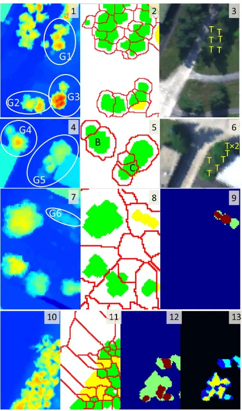
in groups of trees and in forest regions. We show in Fig. 3 four situations and six tree groups with available ground truth results, which will show the differences between these tools together with the their advantages and disadvantages. The images 1-9 of Fig. 3 make it clear that mostly, the moduleW
combined with classification results yields a correct result on individual tree detection. The reason is that mostly two assump-tions hold: 1) in the slightly smoothed airborne laser data, a clear local maximum of the elevation map corresponds to an individ-ual tree and 2) the region border is given either by the shedding line between two components or by the classification result. In the first two rows, groups of trees G1, G3, G4, were successfully delineated and the configurations correspond to the reality.However, if the first assumption does not hold, some trees con-sist of more than one crown and belong to several components. For example, see a tree in the bottom middle of Fig. 3, 7-9. This problem has been noted, to a larger extent, in the high-resolution datasets from multi-view configurations of images. In photogram-metrically generated point clouds of a high resolution (100 points per m2), see, for instance, (Rothermel et al., 2014), a footprint of a big tree usually has many local maxima. To solve this problem, we will implement the multi-scale method of (Persson, 2001) in our future work. Cases when the second assumption fails con-cern the trees that are either occluded completely by other trees – which happens for groups G2 and G5 of Fig. 3) – or for which the local maxima have been over-smoothed. For instance, in the top of images 7-9, Fig. 3, three trees near a building wall were accurately cut; hence,
W
found just one component with a suspi-ciously large eccentricity. Hence, this component has been pro-cessed withH
and two of three trees were detected, see Fig. 3, image 9. In this special case, also the last tree could be detected within the primitive collectionP
. In Fig. 3, bottom row, we see how big components are processed withH
and single trees are selected in a repletion of nested regions. The remaining green components are then analyzed whether they are hills. At this point, we arrive at the next section about the detection and recon-struction of hills. It remains to mention that the results presented in this section are superior to those of (Reitberger, 2010) (< 65%), (Persson, 2001) ( < 68%) and are slightly below those of the local maximum refinement and delineation algorithm (LMRDA) due to (Pouliot et al., 2002) with its best result of 91% of per-pixel de-tection; though the number of trees in the sample, the complexity of situation, and the measure for assessment of accuracy certainly vary in all contributions.8.2 Detection and Reconstruction of Hills
To perform the verification of small hills and earth walls, we first need a reliable ground truth. To obtain it, we applied a pixel-wise supervised classification using hyper-spectral and elevation-based data as well as a support vector machine (Chang and Lin, 2011). The data and the method could seem like an overkill for detection of earth walls, but are necessary for verification. The spectral bands are directly used as hyperspectral features exclud-ing the ones with bad signal-to-noise ratio. Additionally, 20 mor-phological profiles are used as elevation-based features (Benedik-tsson et al., 2005). To combine these features in a meaningful way, we normalize them by removing the mean and dividing them by their standard deviation. For several classes likebuilding,tree, grassand the target classhill, between 400 and 700 pixels are used to train the classifier. Post classification is used to reduce the false alarm rate. Connected components are identified and
Figure 4: View of a urban terrain reconstruction result for the complete dataset. In the bottom part, on the left: A larger fragment with results for hills detection (see text for details); on the right: The corresponding fragment of the DSM.
isolated pixels misclassified as hills are removed. The overlap of the ground truth and our result is depicted in Fig. 4, bottom left. The blue color indicates the false negatives: hills in the ground truth but not detected by our procedure. There are three false negatives: One because of its area and two because of the pla-narity measure (see Sec. 5). Also, there were no false positives. There are ten true positives, such that the results for completeness and correctness are 76% and 100%, respectively. For true posi-tives, we also showed the per-pixels detection results. By dark red, yellow, and orange colors, respectively, we specify the areas of accordance, missed part of a hill, and superfluous part of the hill (which is not a problem, since trees upon the hills are filtered out anyway).
We can conclude from the figure and from the explanations that detection of hills is a complicated job if they are occluded by trees. However, the numbers for completeness and correctness are encouraging; they can be improved in the future by adjusting thresholds or a reasonable integration of other features.
As for the hill reconstruction, the grid size for different hills has remained constant (around 1m), except that for reasons of speed and numerical precision, the number of grid points should remain below 100×100. The smoothness parameter for the functional in (Bulatov and Lavery, 2010, D’Errico, 2005) was chosen around 0.5. No big change of the results occur for moderate (±10% to 20%) changes in these parameters. The main difference is caused by the choice of the reconstruction algorithm. The procedure based on work of (Bulatov and Lavery, 2010) is better suited for modeling regions of both slow and rapid smooth change than the procedure based on (D’Errico, 2005), at cost of computing time.
8.3 First Results on Classification of Trees
We selected 24 trees which were detected as individual trees by
S
andW
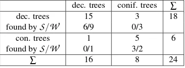
and made following observations, which are also visu-alized in Table 2 and Fig. 5: With an exception of one deciduous tree (C) which is very cramped between the building wall and some other trees, the coniferous are more likely to be modeled by very narrow ellipses or cones. Several kinds of coniferous trees, however, exhibit a large value of the measure from (5). The prob-lem could mostly be observed for trees detected withW
. Hence, one possible explanation could be that the delineation was not clean enough. However, it is obvious that obtaining reliable re-sults for classification of trees by using only one characteristics – tree shape – is hardly possible.9. CONCLUSIONS AND OUTLOOK
Table 1: Behavior for the modules
W
andH
for six example clusters of trees. The second row shows number of trees in the group while the second row shows the complexity level of the situation (trees growing close to each other, under the crones of other trees etc.): Not very challenging (1), challenging (2), and very challenging (3). The lines 3-6 show the absolute and relative numbers of detected individual trees for the methods discussed above. Unfortunately, no ground truth was obtained for Fig. 3, 10-13. Also, delineation of some single trees was not recorded.Cluster nr. 1 2 3 4 5 6 ∑
# Trees 6 3 4 2 7 3 25
# Complexity 2 3 1 3 3 3
-# (
W
) 6 2 3 2 4 1 18In % 100 67 75 100 57 33 72
# (
W
+H
+P
) 6 2 4 2 4 3 21In % 100 67 100 100 57 100 84
Figure 5: Top row: The first three images show selected trees which are approximated by conics as shown in the three images of the bottom row. Top right: Part of the DSM. Bottom right: Two prototypes for tree models.
Table 2: Preliminary results of tree classification
dec. trees conif. trees ∑
dec. trees 15 3 18
found by
S
/W
6/9 0/3con. trees 1 5 6
found by
S
/W
0/1 3/2∑ 16 8 24
the situations where this result is not reliable should be recog-nized and corrected. Recognition (especially with respect to the component analysis based on hotspots detection with ISOL algo-rithm) and reconstruction of such anomalies make up the main contributions of this work. The hotspots detection is applied in order to identify trees upon hills and in other areas where water-shed transform has failed. However, ISOL and MSER have both a number of empiric thresholds. To their further disadvantages with respect to watershed transformation, computation time and necessity to analyze nested components can be added.
We are aware that further theoretical concepts are necessary to analyze and to correct more general cases of misclassification that may theoretically occur (cavities instead of hills, trees growing upon building roofs, and many others) and we will consider it in our future work. Finally, with respect to simulations, even a few tree types with corresponding texture pictures aggravate the interaction if the total number of trees is very large. This is the reason why on the one hand, we want to improve and broaden the classification of trees, which at the moment is based merely on parameters of a conic approximating the point cloud, and on the other hand, we search for a memory-efficient representation of large forest regions in areas less relevant for simulation.
REFERENCES
Abdel-Aziz, Y. and Karara, H., 1971. Direct linear transforma-tion from comparator coordinates into object space coordinates in close-range photogrammetry. Proc. of Symp. on Close-Range Photogrammetry, American Society of Photogrammetrypp. 1–18.
Anderer, C., Thönnessen, U., Carlsohn, M. F. and Klonz, A., 1989. Ein Bildsegmentierer für die echzeitnahe Verarbeitung. DAGM-Symposiumpp. 380–384.
Andersen, H.-E., Reutebuch, S. E. and Schreuder, G. F., 2001. Automated individual tree measurement through morphological analysis of a lidar-based canopy surface model. In:Proc. Interna-tional Precision Forestry Symposium, Seattle, WA, USA, pp. 11– 21.
Bechtel, B., 2007. Objektextraktion von Bäumen aus Luftbildern: Vergleich und Steuerung von Segmentierungsverfahren zur Vor-bereitung eines Expertensystems. PhD thesis, Universität Ham-burg, HamHam-burg, Germany.
Benediktsson, J. A., Palmason, J. A. and Sveinsson, J. R., 2005. Classification of hyperspectral data from urban areas based on ex-tended morphological profiles.IEEE Transactions on Geoscience and Remote Sensing43(3), pp. 480–491.
Bulatov, D. and Lavery, J. E., 2010. Reconstruction and texturing of 3D urban terrain from uncalibrated monocular images usingL1 splines.Photogrammetric Engineering & Remote Sensing76(4), pp. 439–449.
Bulatov, D., Häufel, G., Meidow, J., Pohl, M., Solbrig, P. and Wernerus, P., 2014. Context-based automatic reconstruction and texturing of 3D urban terrain for quick-response tasks. ISPRS Journal of Photogrammetry and Remote Sensing93, pp. 157 – 170.
Chang, C.-C. and Lin, C.-J., 2011. LIBSVM: A library for sup-port vector machines. ACM Transactions on Intelligent Systems and Technology (TIST)2(3), pp. 1–27.
D’Errico, J., 2005. Surface fitting using gridfit.MATLAB central file exchange.
Eysn, L., Hollaus, M., Lindberg, E., Berger, F., Monnet, J.-M., Dalponte, M., Kobal, M., Pellegrini, M., Lingua, E. and Mongus, D., 2015. A benchmark of LiDAR-based single tree detection methods using heterogeneous forest data from the Alpine space. Forests6(5), pp. 1721–1747.
Hirschmüller, H., 2008. Stereo processing by semi-global match-ing and mutual information.IEEE Transactions on Pattern Anal-ysis and Machine Intelligence30(2), pp. 328–341.
Horn, H. S., 1971.The adaptive geometry of trees. Vol. 3, Prince-ton University Press.
Kaartinen, H., Hyyppä, J., Yu, X., Vastaranta, M., Hyyppä, H., Kukko, A., Holopainen, M., Heipke, C., Hirschmugl, M., Mors-dorf, F. et al., 2012. An international comparison of individual tree detection and extraction using airborne laser scanning. Re-mote Sensing4(4), pp. 950–974.
Koch, B., Heyder, U. and Weinacker, H., 2006. Detection of individual tree crowns in airborne lidar data. Photogrammetric Engineering & Remote Sensing72(4), pp. 357–363.
Lafarge, F. and Mallet, C., 2012. Creating large-scale city models from 3D-point clouds: a robust approach with hybrid representa-tion.International Journal of Computer Vision99(1), pp. 69–85.
Matas, J., Chum, O., Urban, M. and Pajdla, T., 2002. Robust wide baseline stereo from maximally stable extremal regions.Proc. of British Machine Vision Conferencepp. 761–767.
Persson, A., 2001. Extraction of individual trees using laser radar data. Department of Signals and Systems, Chalmers University of Technology, Göteborg, Sweden.
Pollock, R. J., 1996. The automatic recognition of individ-ual trees in aerial images of forests based on a synthetic tree crown image model. PhD thesis, Concordia University, Montreal, Canada.
Pouliot, D., King, D., Bell, F. and Pitt, D., 2002. Automated tree crown detection and delineation in high-resolution digital camera imagery of coniferous forest regeneration. Remote Sensing of Environment82(2), pp. 322–334.
Reitberger, J., 2010. 3D-Segmentierung von Einzelbäumen und Baumartenklassifikation aus Daten flugzeuggetragener Full Waveform Laserscanner. PhD thesis, TU Munich, Munich, Ger-many.
Rothermel, M., Haala, N., Wenzel, K. and Bulatov, D., 2014. Fast and robust generation of semantic urban terrain models from UAV video streams. In:Proc. of 22nd International Conference on Pattern Recognition, ICPR, pp. 592–597.
Secord, J. and Zakhor, A., 2007. Tree detection in urban regions using aerial lidar and image data. IEEE Geoscience and Remote Sensing Letters4(2), pp. 196–200.
Straub, B.-M., 2003. Automatic extraction of trees from aerial images and surface models. The International Archives of the Photogrammetry, Remote Sensing and Spatial Information Sci-ences34(3/W8), pp. 157–166.