FULLY AUTOMATED GIS-BASED INDIVIDUAL TREE CROWN DELINEATION
BASED ON CURVATURE VALUES FROM A LIDAR DERIVED CANOPY HEIGHT
MODEL IN A CONIFEROUS PLANTATION
R. J. L. Argamosa a,* E.C. Paringit a, K.R. Quinton b, F. A. M. Tandoc a, R. A. G Faelga a, C. A. G. Ibañez a, M. A. V. Posilero a, G. P. Zaragosa a
a Phil LiDAR 2 - Project 3: Forest Resources Extraction from LiDAR Surveys. University of the Philippines Diliman, Quezon City (regi.argamosa, paringit, tandoc.fe, reginefaelga, i.carlynann, markposi, gio.zaragosa)@gmail.com
b Phil LiDAR 1 – Hazard Mapping of the Philippines using LiDAR. University of the Philippines Diliman, Quezon City ([email protected])
Commission VIII, WG VIII/7
KEY WORDS: Crown Delineation, Canopy Height Model (CHM), Local Maxima, Curvature, Slope, Thiessen Polygons
ABSTRACT:
The generation of high resolution canopy height model (CHM) from LiDAR makes it possible to delineate individual tree crown by means of a fully-automated method using the CHM’s curvature through its slope. The local maxima are obtained by taking the maximum raster value in a 3 m x 3 m cell. These values are assumed as tree tops and therefore considered as individual trees. Based on the assumptions, thiessen polygons were generated to serve as buffers for the canopy extent. The negative profile curvature is then measured from the slope of the CHM. The results show that the aggregated points from a negative profile curvature raster provide the most realistic crown shape. The absence of field data regarding tree crown dimensions require accurate visual assessment after the appended delineated tree crown polygon was superimposed to the hill shaded CHM.
1. INTRODUCTION
Tree crowns provide many ecological benefits such as the reduction of greenhouse gases, water improvement (filtration and retention), and reduction of storm water runoff. (Troxel, et. al., 2013). The amount or rate of rainfall and light interception can also be determined by tree crowns. Forest soil is also benefitted as it contributes to forest litter accumulation and can also determine the soil moisture and loss (Husch, et al., 2003 as cited by Perez et al., 2006)
Aside from being a complement of the net primary production, tree crown dimensions depict the general health of the tree (Perez, et al. 2006). Several allometric equations suggest that there is a strong correlation between tree crown and growth thus, tree crown dimension is usually used for quantifying tree growth. (Kozlowski et al., 1991 as cited by Perez et. al., 2006).
Nevertheless , getting the dimensions and actual forms of tree crowns is tedious that it is usually left out in most forest inventory. Measuring tree crowns in the field is likewise very prone to subjectivity especially during the measurement of the crown’s extent. . Instead, allometric equations are used yet the estimated values may result in inaccurate models of tree crowns.
The objective of this study is to create a GIS-based method that will automatically delineate individual tree crowns in a coniferous forest plantation. The study also aims to serve as an acceptable substitute for tree crown delineation that can only be done by algorithms offered by expensive proprietary object-based image processing software.
2. MAIN BODY
2.1 Materials and Methods
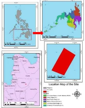
2.1.1 Site Description: The study area is located in Malitbog, Bukidnon, Philippines between geographical coordinates 124° 59' 26.9052" N, 8° 29' 22.2504" E and nestled at elevation 970 m – 1000 m. The landscape is heavily dominated by a tree species known as Caribbean Pine (Pinus caribaea) and some Eucalyptus trees (Eucalyptus deglupta). The trees are planted in 3 m x 3 m arrangement . Extraction of the Caribbean Pine’s sap to produce resins is the main purpose of the stand. The Bukidnon Forest, Inc. operates the area as a joint forest business venture between the Philippines and New Zealand (bukidnonforestinc, 2014). Figure 1 shows the location map. The DTM (digital terrain model) and CHM (Canopy Height Model) are shown in Figure 2. The 3D models of CHM and DTM are shown in Figure 3.
Figure 1. Location Map of the Coniferous Plantation
Figure 2. DTM (left) and CHM (right)
Figure 3. 3D Model of DTM (left) and CHM (right)
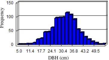
2.1.2. Field Inventory: Field inventory survey was conducted from February 15 – 24, 2015 to come up with a contiguous two-hectare plot. The diameter at breast height (DBH) and tree height were obtained. In addition, precise location of each tree was determined by using GPS control and total station. The measurement of the tree crown was not done to conform with the purpose of the field inventory which is to calibrate LiDAR metrics to estimate the DBH/Biomass/Carbon Stock and Canopy Cover. Figures 4 and 5 show the histogram of DBH and tree height, respectively. Tables 1 and 2 show the the descriptive statistics for DBH and tree height, respectively.
Figure 4. Histogram of DBH (cm) values
Figure 5. Histogram of Tree Height (m) values
Descriptive Statistics Values
Table 1. Computed descriptive statistics for DBH (cm) values
Descriptive Statistics Values
Table 2. Computed descriptive statistics for Tree Height (m) values
2.1.3. LiDAR Data Processing: LiDAR data was generated from flight 388G, conducted on August 16, 2013 with a flying height of 303.69 meters above sea level. The recorded pulse density is 1.99 per square meters.
Generating a good CHM is necessary in an automated crown delineation. A good CHM means that the pits should be removed or minimized. Khosravipour et. al. (2012) defined the pits as the first returns originated far below the canopy which is caused by laser beam’s deep penetration through the canopy’s foliage and the presence of multiple laser beams with close x and y values but significantly different z values. These anomalies will lead to pits when rasterized. The possible source of errors in CHM creation is eliminated by using the pit-free algorithm (Khosravipour op.cit)
The LiDAR processing software LAStools (Version 160110; Isenburg, 2015) was used to create the pit-free CHM. Following the algorithm, the classified LAS was normalized with respect to elevation values. The produced LAS contains the actual z values of the objects above ground (trees). From the normalized LAS, LiDAR points with the highest z-values in a 0.5 m resolution were selected. The beam size of each selected LiDAR points were replaced by a disk plate with a radius of 0.05. The LAS was then rasterized into six rasters with unique threshold values. The first rasterization was done by triangulating all first
F
Normalized LAS
Highest z values in a cell
•Rasterization of all points
•Rasterization of points with z values >= 2 m.
•Rasterization of points with z values >= 5 m.
•Rasterization of points with z values >= 10 m.
•Rasterization of points with z values >= 15 m.
•Rasterization of points with z values >= 20 m.
Merging into one raster (CHM)
19.44 31.65
Generate Local Maxima
Computes curvature points
Create polygons
Append created polygons returns. The second to sixth rasterization was done by
triangulating points with a height greater than or equal to 2 m, 5 m, 10 m, 15 m, and 20 m, respectively. All created rasters will be stacked into one. Figure 6 shows the normalized LAS while Figure 7 shows the diagram of the pit-free algorithm workflow.
Figure 6. Normalized LAS (LiDAR Point Cloud)
Figure 7. Pit-free algorithm workflow
The algorithm produces a clean and pit-free CHM as shown in Figure 8.
Figure 8. The resulting CHM of the pit-free algorithm
2.1.4. Crown Delineation: The proposed crown delineation method can be summarized into four parts as shown in Figure 9. The first part is the generation of local maxima to determine individual trees. The second part computes for the curvature
points while the third part converts the points to polygons and smoothens the edges. The fourth part appends all of the polygons created.
Figure 9. The general workflow of crown delineation algorithm
Taking the CHM as an input, pixels with elevation values greater than or equal to 5 m were extracted. The maximum value in a 3 m x 3 m cell was obtained from these rasters. To get the individual pixels that represents the local maxima, the output raster was calculated using the formula:
LM=Con (CHM==FS, CHM) (1)
where Con=conditional function CHM=Input CHM
FS=maximum values in a 3 m x 3 m cell LM=local maxima
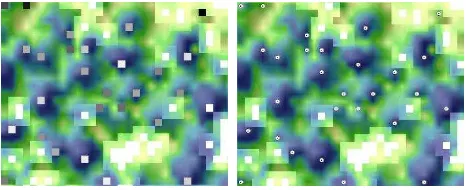
The output of the local maxima raster was converted into points. Figures 10, and 11 show the output of the processes stated above.
Figure 10. Height values greater than or equal to 5 m (left) and the maximum values in a 3 m x 3 m cell (right)
Figure 11. CHM overlaid with the local maxima (left) and the local maxima to points overlaid in the CHM (right).
The second part takes the CHM as an input to compute for the slope. Figure 12 shows the surface scanning window for ArcGIS’ computation of slope.
According to Rodriguez and Suarez in 2010 and as cited in ArcGIS (Version 10.3; ESRI, 2016) the slope is computed as:
“…the maximum rate of change in a value from that cell to its neighbours. Basically, the maximum change in elevation over the distance between the cell and its eight neighbours identifies the steepest downhill descent from the cell”.
Figure 12. Surface scanning window (ArcGIS Version 10.3; ESRI, 2016)
The slope algorithm used by ArcGIS 10.3 is shown below in detail:
First, the rate of change in x and y direction for e is computed as:
Δ x = ((c + 2f + i) - (a + 2d + g) / (8 * 3) (2) Δ y = ((g + 2h + i) - (a + 2b + c)) / (8 * 3) (3)
The slope (rise/run) is computed by taking the Δ x and Δ y.
m = √ ([Δ x] 2 + [Δ y] 2) (4)
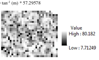
The slope is converted into degrees by getting the product of the arc tan of the slope and the result of 180 over Pi. Figure 13 shows the raster of the generated slope.
m° = tan-1 (m) * 57.29578 (5)
Figure 13. Generated slope raster
The generated slope was used to compute for the curvature and is shown in figure 14. The equation for computing the curvature of the slope is
Curvature = -2(D + E) * 100 (6)
where D = [(Z4 + Z6) /2 - Z5] / L2 E = [(Z2 + Z8) /2 - Z5] / L2
Figure 14. Curvature values Diagram (ArcGIS Version 10.3; ESRI, 2016)
The profile curvature was computed by getting the curve parallel to the maximum slope. The output of the profile curvature can be grouped into the positive, negative, and zero values. Since the structure of a pine tree is convex, the negative profile curvature was used since the negative values depicts the upward convex curve at that cell (ArcGIS Version 10.3; ESRI, 2016). The resulting raster was converted into points. The illustration of a negative profile curvature is shown in Figure 15 while the converted points is shown in Figure 16.
Figure 15. Negative profile curvature (left) and a Pinus carribaea species (right)
Using the local maxima as input, a thiessen polygon was created. Thiessen polygons creates a unique and non-overlapping polygons on the nearest point. Thus, every thiessen polygon will surround the nearest and unique point. Each polygon is created by triangulating the points (red line in the figure below). Each line created will be passed through by a bisector line (black line in the figure below) and these represents the thiessen polygons. (Gitta, 2013). Figure 17 shows the thiessen polygons overlaid in the CHM.
Figure 16. Construction of a Thiessen Polygon The International Archives of the Photogrammetry, Remote Sensing and Spatial Information Sciences, Volume XLI-B8, 2016
Figure 17. Negative profile curvature converted to points (left) and Thiessen polygons (right)
The thiessen polygon was intersected to the negative profile curvature. The points that intersected a common polygon will be aggregated to create a polygon representing the crown. Edges will also be smoothened. Figure 18 shows the negative profile curvature, its intersection with the thiessen polygon, and the aggregated and smoothened polygon that represents the crown extent.
Figure 18. Features overlaid in the CHM: Negative profile curvature (left), intersected thiessen polygon (right), final crown
extent (bottom).
The final step is to append all the polygons created into a one shape file.
2.2. Results and Discussion
Figure 19 shows the final output of the algorithm while Figure 20 shows when it is overlaid in the CHM.
\
Figure 19. The final output of the algorithm
Figure 20. The final output overlaid in the CHM
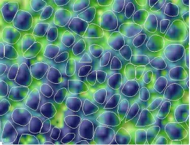
Most of the output of the proposed algorithm were able to accurately delineate tree crowns as shown in Figure 21.
Figure 21. A portion of the area with properly segmented crown
Some of the delineated tree crown is over segmented as shown in Figure 22.
Figure 22. A portion of the area with over segmented crown The International Archives of the Photogrammetry, Remote Sensing and Spatial Information Sciences, Volume XLI-B8, 2016
3. CONCLUSION
The proposed algorithm was able to delineate crown polygons. Visually speaking, the delineation was able to represent individual tree crowns accurately. Errors can be caused by the inaccurate representation of individual trees using local maxima since some highest point does not necessarily mean that it belongs to one tree only.
The use of values of a negative profile curvature accurately mark the descent of the edges of the coniferous tree. Still , since the aggregation distance is the same for all trees, smaller trees sometimes represent bigger crown extent and bigger trees sometimes represent smaller crowns. Further addition of conditional statements per tree size should be considered in order to reduce the bias.
4. ACKNOWLEDGEMENTS
This work was supported by Philippine Council for Industry, Energy and Emerging Technology Research and Development of the Department of Science and Technology (PCIEERD-DOST), under the Nationwide Detailed Resources Assessment Using LiDAR (Phil-LiDAR 2), Project 3: Forest Resources Extraction from LiDAR Surveys (FRExLS). Recognition is given to Disaster Risk and Exposure Assessment for Mitigation (DREAM) and Phil-LiDAR 1 Program. Acknowledgement is also given to Central Mindanao University (CMU) and Bukidnon Forest Incorporated (BFI) for their assistance the field works.
5. REFERENCES
Gitta. 2013. Thiessen Polygon. Geographic Information
Technology Training Alliance.
http://www.gitta.info/Accessibilit/en/html/UncProxAnaly_learn ingObject4.html
Khosravipour, A. et. al., 2013. Development of an Algorithm to Generate a LiDAR Pit-Free Canopy Height Model. Silvilaser 2013 (SL2013-030). pp. 125-126.
Perez, J.J. et. al. 2006. Tree Crown Structure in a Mixed Coniferous Forest in Mexico. Conference on International Agricultural Research for Development. pp. 1-7.
Rodriguez, J.G. et. al. 2010. Comparison of Mathematical Algorithms for Determining the Slope Angle in GIS Environment. Aqua-LAC (Vol 2). pp. 78-82.
Troxel, B. et. al., 2013. Relationships Between Bole and Size for Young Urban Trees in the North-eastern USA. Urban
Forestry and Greening (UFUG-25329).
http://dx.doi.org/10.1016/j.ufug.2013.02.006. pp. 1-10.
Widlowski, J.L. et. al .2003. Allometric Relationships of Selected European Tree Species. EC Joint Research Centre (EUR 20855 EN). pp. 38-42.
6. APPENDIX
The following texts show the code written in Python language that utilizes several arcpy functions to delineate tree crowns as stated in this paper. The script can only be executed outside the ArcGIS software and requires that the CHM and the arcpy script is contained in the same folder.
import arcpy, os, shutil
ext1=ExtractByAttributes(self.chm, sql) ext1.save(self.ext)
fs1=FocalStatistics(self.ext, NbrRectangle(spc, spc, "CELL"),"MAXIMUM", "NODATA")
fs1.save(self.fs)
rascalc=Con(Raster(self.ext)==Raster(self.fs),Raster(self.ext)) The International Archives of the Photogrammetry, Remote Sensing and Spatial Information Sciences, Volume XLI-B8, 2016
rascalc.save(self.rc)
arcpy.CheckInExtension('Spatial')
arcpy.RasterToPoint_conversion(self.rc, self.pt, '#') arcpy.Integrate_management(self.pt,self.xy_tol)
def curv_pts(self):
print 'generating negative profile curvature' arcpy.CreateThiessenPolygons_analysis(self.pt, self.thie,"ALL")
arcpy.CheckOutExtension('3D')
arcpy.Slope_3d(self.ext,self.slope, "DEGREE",1) arcpy.Curvature_3d (self.slope,self.curv, 1, self.prof,"#") arcpy.CheckInExtension('3D')
arcpy.RasterToPoint_conversion(self.prof, self.prof1, '#')
arcpy.Select_analysis(self.prof1,self.rtpprof,where_clause="""" GRID_CODE" < 0""")
arcpy.Clip_analysis(self.rtpprof,self.thie,self.clip) arcpy.Intersect_analysis([self.thie,self.clip],self.int, "ALL","","INPUT")
arcpy.Dissolve_management(self.int,self.diss, 'FID_thie','#', "MULTI_PART","DISSOLVE_LINES") def smooth1(self):
print 'smoothing polygons' fc3=self.diss
field3="FID_thie"
cursor3=arcpy.SearchCursor(fc3) x=0
for row3 in cursor3: x+=1
row3.getValue(field3)
arcpy.MakeFeatureLayer_management(fc3, "lyr") arcpy.SelectLayerByAttribute_management("lyr", "NEW_SELECTION",\
"FID_thie="+str(row3.getValue(field3))) itername=string.zfill(x,5)+'.shp'
print str(x)+' '+'crowns created!' arcpy.AggregatePoints_cartography('lyr', self.aggre+itername,self.size)
CA.SmoothPolygon(self.aggre+itername, self.smooth+itername, "PAEK", 3)
def append(self):
print 'appending shapefiles'
utm=arcpy.SpatialReference("WGS 1984 UTM Zone 51N")
arcpy.CreateFeatureclass_management(ws, self.name, "POLYGON", "#", "DISABLED",\
"DISABLED", utm) env.workspace=self.add
listindv=arcpy.ListFeatureClasses()
arcpy.Append_management(listindv, ws+'\\'+self.name, "NO_TEST","#","#")
print 'Done!' c=crown() c.inchm() c.curv_pts() c.smooth1() c.append()