CONSISTENT MULTI-VIEW TEXTURING OF DETAILED 3D SURFACE MODELS
K. Davydovaa, G. Kuschka, L. Hoegnerb, P. Reinartza, U. Stillab
aRemote Sensing Technology Institute, German Aerospace Center (DLR), D82234 Wessling, Germany
[email protected], (georg.kuschk, peter.reinartz)@dlr.de b
Photogrammetry & Remote Sensing, Technische Universitaet Muenchen (TUM), Arcisstr. 21, 80333 Munich, Germany-(stilla, ludwig.hoegner)@tum.de
KEY WORDS:Multi-texturing, 3D model, Large-scale, Aerial images, MRF, Seam visibility, Urban
ABSTRACT:
Texture mapping techniques are used to achieve a high degree of realism for computer generated large-scale and detailed 3D surface models by extracting the texture information from photographic images and applying it to the object surfaces. Due to the fact that a single image cannot capture all parts of the scene, a number of images should be taken. However, texturing the object surfaces from several images can lead to lighting variations between the neighboring texture fragments. In this paper we describe the creation of a textured 3D scene from overlapping aerial images using a Markov Random Field energy minimization framework. We aim to maximize the quality of the generated texture mosaic, preserving the resolution from the original images, and at the same time to minimize the seam visibilities between adjacent fragments. As input data we use a triangulated mesh of the city center of Munich and multiple camera views of the scene from different directions.
1. INTRODUCTION 1.1 Motivation
3D computer visualization of the real world plays an increasing role in today’s information society. It has already found its way into several applications: street view perspectives on maps (e.g. Google-Earth); virtual 3D city models, which are used for ur-ban planning and reconstruction, computer gaming (Frueh et al., 2004); real-time environmental and physical simulations for dis-aster management; 3D scanning for virtual cultural heritage con-servation (Alj et al., 2012). However, for all these applications the accurate and realistic appearance of the objects is required. That could be achieved by texture mapping.
Texture mapping can be generally defined as a computer graphic technique used to map a two-dimensional (2D) texture space (im-ages) to a three-dimensional (3D) model space. A number of images should be taken to reconstruct the textured geometrical model, because a single image cannot capture all parts of a 3D model. The surface of a 3D model is defined as a set of poly-gons (commonly triangular mesh), so that the coordinates of each polygonal vertex can be found from the images on the assump-tions that the images and the 3D model are registered within a global coordinate system. In other words, each image can be back-projected onto the surface to generate a texture fragment. The combination of these texture fragments yield the so-called texture map.
From different types of images one can extract different infor-mation. Texturing the 3D building models from thermal infrared (IR) images can be used for the thermal inspections (Iwaszczuk et al., 2011) and monitoring (Kolecki et al., 2010), together with heat leakage detection on building facades (Hoegner and Stilla, 2009). However, the low resolution and small field of view of IR cameras are serious problems, when models are textured with IR images (Hoegner and Stilla, 2009). Using multispectral images for texturing 3D models allows quantitative evaluation or study of the materials lying on the object surface (Pelagottia et al., 2009). In this case the problem is addressed only to texture small test sites. With the progress in computer systems and algorithmic improvements it becomes possible to texture the digital object surfaces with texture information from photographic images to
achieve a high degree of realism of computer generated digital models. Therefore, in our paper we aim to texture a real-world and large-scale 3D city model by applying the high-resolution aerial photographic images.
1.2 Related Work
In the ideal case, i.e. same lighting conditions in the multiple camera views, perfect perpendicular looking angles and ideal ge-ometric model, the texturing of a real object from photographic images is straightforward and seamless. However, these condi-tions are difficult (in practice nearly impossible) to achieve and one has to overcome the problems connected with it. In the last few years, several texturing methods of 3D models from multi-ple images were developed to solve these problems. Some tech-niques suggest to blend (pixel-wise color averaging) the textures from several images per face to build a texture map. First in-troduced in (Debevec et al., 1996) the View-Dependent texture-mapping method renders the 3D models by a view-dependent combination of images. For a given view, the textures are typi-cally blended based on the closest position of two neighbor views from the view-point (the smallest angle between the face normal and the view direction of the input camera). To smooth the visi-ble seams due to assigning the different images to the neighboring faces, weighted averaging is applied. The authors in (Wang et al., 2001) compute the correct weights for blending by image pro-cessing. The steps of reconstruction, warping, prefiltering, and resampling in order to warp reference textures to the desired po-sition are applied afterwards (Wang et al., 2001). This is then treated as a restoration problem and is solved to construct a fi-nal optimal texture. An innovative texture mapping method was proposed in (Baumberg, 2002). The author decomposes each in-put image into a low frequency band camera image and into a high frequency band camera image. The images are blended af-terwards in each frequency domain independently and the results are combined to generate a final texture mosaic. However, in all these approaches, blending the textures from several images per face to build a texture map leads to ghosting and blurring arti-facts.
the best image is identified as the one on which the projection of all triangle vertices exist and the angle between the direction of the vertex normal and the camera is the smallest. To produce a smooth join when a mesh face is on the adjacency border between different observed images, the weighted blending of correspond-ing adjacent image sections is applied afterwards, followed by a piecewise local registration procedure, further improving the ac-curacy of the blending process. The authors in (Frueh et al., 2004) apply texture mapping on an existing 3D city model from the im-ages obtained at oblique angles. They propose to find the optimal image for mapping every single triangle of the 3D geometrical model based on parameters such as occlusion, resolution, sur-face normal orientation and coherence between adjacent sur-faces. In (Iwaszczuk et al., 2013) quality for the “best” texture selection is measured as function of occlusion, angles between normal of the investigated face and direction to the projection center and its distance to the projection center. However, this algorithm gives only the reference texture for each face to the frame or frames where this face has the best quality. Therefore this procedure can be done prior to the texture extraction.
Due to the selection of the single “best” image for each triangle the seams are not avoided if the images are taken under different illumination conditions. The method proposed by (Lempitsky and Ivanov, 2007) is formulated as a discrete labeling problem, where the images are related to labels, which should be assigned to each mesh face. The solution to the problem is connected to a Markov Random Field (MRF) energy minimization problem with two terms. The first term, called data term, describes the quality of the given texture. This criterion is based on the angle between the local viewing direction of the corresponding view and the face normal. The second term, called regularization term, defines the consistency between neighboring faces. The authors in (Allene et al., 2008) proposed to calculate the data term related to the pro-jection area of the 3D triangle in image space. A method in (Gal et al., 2010) introduces the assignment of the faces with a set of transformed images, which compensate the geometric errors, and, applying Poisson blending, removes lighting variations. The methodology proposed in this paper is based on the Markov Random Field approach which allows not only the selection of one best view per face using a special criterion, but also simul-taneously apply regularization on the texture assignment to min-imize seam visibilities on the face boundaries. Additionally, it helps to avoid the intensity blending as well as image resampling on all stages of the process (Lempitsky and Ivanov, 2007). This guarantees that the resolution of the resulting texture is basically the same as in the original views.
2. METHODOLOGY 2.1 Energy function formulation
To reconstruct the textured geometrical object a number of im-ages should be taken, as a single image cannot capture all parts of a 3D model. Best texture selection for the problem is based on the idea discussed in (Kuschk, 2013). However, to create a single coherent texture, additional smoothness constraints for the merged texture map are required. The approach for the process in this paper is considered as a discrete labeling problem, the so-lution of which is provided by MRF energy optimization. On a given set of images{I1, . . . , In}, providing the texture
in-formation, each triangular face{t1, . . . , tm}of the 3D model is
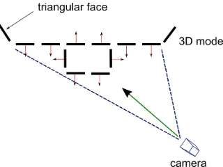
projected. We check whether a triangular face looks towards a given camera as it is shown in Figure 1 and store its 2D coor-dinates. Because triangles may be visible in several images, we aim to find the image with the “best” texture for these faces. This problem is formulated as a discrete labeling problem, where the
Figure 1. Texture determination. Red arrows represent the nor-mal vectors of each triangle.
Figure 2. Geometry of the angle between a face’s normal vector and the looking vector of the camera.
images are related to the labelsL={l1, . . . , ln}, which should
be assigned to each triangular face taking into account additional information about the interaction between the neighboring trian-gles. We then define the texture mosaic byF={f1, . . . , fm},
which describes the texturing (labelling) of all triangular facesti.
Obviously, not from all images a given triangle could be seen equally. The criterion to measure the quality of a triangle texture observed in each imageIjis based on two parameters:
1. The angle between a face’s normal vector and the looking vector of the camera (αdif f). The larger the angle (closer to
180◦
) the more preferable the texture from that image (see Figure 2);
2. The visible area of the projected triangle in the image. Let us denote the projected area of triangleti in image Ij as
P(ti, Ij). The visible area parameter of this projected area
is defined asV is(P(ti, Ij)). The bigger this value the more
preferable the texture from that image (as it allows for finer texture details).
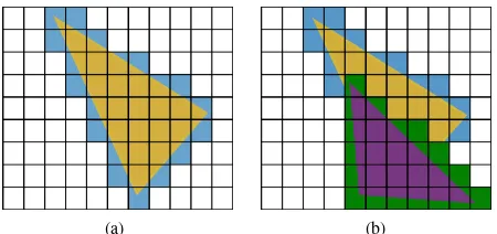
To compute the visible areaV is(P(ti, Ij))of the triangle, az
-buffering approach is used. The main idea of this approach states to rasterize and sort all triangular faces of the 3D model accord-ing to the distance from the camera view. The algorithm starts with projecting each triangular face to the image plane, begin-ning from the furthest face. Then for each interior pixel of the triangular face the corresponding depth value is computed. We check if the depth value of the current pixel in image-space is smaller than the corresponding value in the z-buffer and assign to this pixel a unique identifier (the index of the currently processed triangle). When the pixel is farther away than the old one, no ac-tion is taken. After processing all triangular faces, the visibility of each triangular face is computed using the previously assigned unique identifiers per pixel.
The number of pixels of each fully or partially visible triangular face in the rendered image is calculated as shown in Figure 3a and 3b correspondingly. The set of visible pixels for the yellow triangle in both Figures 3 is defined by the grid area of blue color around it. In mathematical notation, this parameter for visibility can be written as following:
(a) (b)
Figure 3. Determining the number of visible pixels (blue) for the yellow triangle. (a) Fully visible triangle. (b) Partially visible triangle.
Finally, the two quality measurementsαdif fandV is(P(ti, Ij))
are combined together to generate the criterion for the best texture per triangular face defined as:
score(ti, Ij) =αdif f(ti, Ij)·V is(P(ti, Ij)) (2)
which is larger for triangles with better quality.
Applying only this criterion to texture the 3D model will show visible seams between the neighboring triangles if they are tex-tured from images taken under different lighting conditions. To penalize these seams, but at the same time maximizing the visual quality of the triangles for each possible combinations of texture information in the mosaic, MRF energy minimization with two terms is applied:
E(F) =Edata(F) +λ·Eprior(F). (3)
The first term considers the constraints related to the data by en-forcing the solution to be consistent with the observations. If we define the label assigned to each face asfithe first term is then
generated as:
whereN1is a normalization constant.
The second term reflects the interactions between adjacent trian-gles. In this paper it is based on matching the color informa-tion of these adjacent triangles. Measuring the color similarity of adjacent triangles is done based on the triangle’s visible pixels in the image, computing the average RGB color per triangle as
¯
one of the visible pixels of a triangular facetiin imageIj. For
adjacent faces, which share one edge, the seam visibility is then measured by Euclidean distance in RGB color space:
Eprior(F) =
Figure 4. Different types of pairwise regularization terms. (a) The linear regularization function without truncation constant (T = 0). (b) The linear regularization function with truncation constant(T
6=0), stopping the increasing penalty of color differences above a given threshold.
whereTis a truncated constant,Nis a set of nodes andV(fi, fj)
is a potential function assigned between nodesfiandfj. The
re-sults are normalized with constantN2 between [0,1]. In other words, the closer a color metric is to 0, the less visible seam be-tween adjacent triangular faces. The abovementioned truncation constantT in regularization termEprior(F)was introduced in
order to preserve very strong color boundaries between adjacent regions arising from truly color differences. This parameter en-forces the labelingFto keep a few regions with significant varia-tions of labels among neighboring sites (Veksler, 2007) (see Fig-ure 4). This property is typically calleddiscontinuity-preserving. Finally, combining the presented functions and inserting them into Equation (3), the overall energy function is computed as:
E(F) =− 1
MRF probabilistic models solve discrete labeling problems via energy minimization, which is equivalent to finding a MAP esti-mation of the labelingF={f1, . . . , fm}:
ˆ
F= arg max F
E(F). (10)
For minimization of our energy function within a MAP-MRF framework a graph cut algorithm is chosen. The main goal of the method is to construct a specialized graph for the energy func-tion to be minimized such that the minimum cut on the graph also minimizes the energy either globally or locally (Boykov et al., 2001), (Kolmogorov and Rother, 2006). The minimum cut is computed very efficiently by maximum flow algorithm due to their equivalence stated by the Ford and Fulkerson theorem (Ford and Fulkerson, 1962).
Figure 5. Example of an aerial image of the inner city of Munich.
Figure 6. Triangulated digital surface model.
label. The swap is a move from current labelingFto new label-ingF’in one iteration, when some sites ofαlabels inFbecome βlabels inF’and some sites ofβlabels inFbecomeαlabels inF’. The expansion is a move from current labelingFto new labelingF’in one iteration, when a set of labels inFchanged to αlabel. As a result, the problem is reduced to binary labelling (α andβ), which is solvable exactly with graph cut. Applying the α-expansion andα−β-swap algorithms we search for the best label for each triangular face and at the same time penalizing the seam visibilities between neighboring faces.
3. DATA
For the multi-view texturing of geometrical objects aerial image data of the inner city of Munich was taken, using the 3K+ camera system from (Kurz et al., 2007). The distance from the camera to the scene is about 2 km, with a ground sampling distance (GSD) of about 0.2 m. The triangulated DSM and 4 images to texture it are the input parameters for this work (see Figure 5 and 6). The images are chosen in such a way that each area of the scene is vis-ible at least from one image. The DSM has a size of 2000×2000 pixels and covers an area of 400×400m.
The implementation is done using the graph cut minimization software provided by (Szeliski et al., 2006), using the libraries provided by (Boykov et al., 2001), (Boykov and Kolmogorov, 2004) and (Kolmogorov and Zabin, 2004).
4. RESULTS
In this section the proposed fully automatic method for creating a textured 3D surface models is validated under different condi-tions. We vary the two parameters in Equation (9): The truncation constantTand the balancing parameterλ.
In order to compare the roles of the two terms in energy func-tion in Equafunc-tion (9) we start withλ= 0. In this case the second
(a)
(b)
Figure 7. Textured inner city Munich model. (a) Textured city model for λ = 0.0. (b) Textured city model forλ = 0.5 (α -expansion algorithm,T= 0).
(regularization) term does not influence the results. To each trian-gle the texture with the best quality value is assigned without any smoothness constraints. The result is demonstrated in Figure 7a. It can be seen that texturing the model based only on the quality parameter (data term) leads to so-called patchy or noisy results. Next, we take the regularization term in Equation (9) into account and run theα-expansion forλ= 0.5 andT = 0 (see Figure 7b). We can see the significant improvements of the texture mosaic: the texture information looks sufficiently smooth. However, for such large-scale model the differences betweenα-expansion and α−β-swap algorithms can not be visually distinguished. There-fore, we present the result for influence of theλparameter only for the expansion algorithm.
sig-nificant variations of labels among neighboring triangles. There-fore, we can see the obvious texture improvement of the resulting model. However, in Figure 8b we still can see the texture distor-tion between the pedestrian zone and the building. This can be associated with geometrical inaccuracies in the model.
(a) (b)
(c) (d)
Figure 8. Selected areas of the textured city model withλ= 0.5 (using theα-expansion algorithm). (a)T= 0; (b)T= 0.1; (c)T= 0; (d)T= 0.1
(a) (b)
(c) (d)
Figure 9. Selected areas of the textured city model withλ= 0.5 (using theα−βswap algorithm). (a)T= 0; (b)T= 0.1; (c)T= 0; (d)T= 0.1
Now we are turning to theα−βswap algorithm. Here we use the same parameter values as for theα-expansion algorithm. The overall results look similar to theα-expansion algorithm (see Fig-ure 9). If we examine the building’s facade in FigFig-ure 9a we see that it is totally blurred and the building in Figure 9c is blurred partially, if the truncation constantTis equal to 0. The reason is the same as was described above for theα-expansion algorithm. Now, turning to the situation when the truncation constantT = 0.1, we can see the obvious texture improvement of the resulting model (see Figure 9b and 9d). This happened again due to the pa-rameter’s ability to enforce the labelingFto keep a few regions with significant variations of texture information among them.
Expansion Swap
ncycles
time
(sec) ncycles
time (sec)
T=0
λ= 0.1 7 173.08 7 185.17
λ= 0.5 6 148.41 5 139.89
T=0.1
λ= 0.1 6 136.41 6 205.09
λ= 0.5 6 119.15 6 222.05
Table 1. Textured city model characteristics forα-expansion and α−βswap algorithms: Number of cycles the algorithm takes to converge (ncycles); Time the algorithm takes to converge in
seconds.
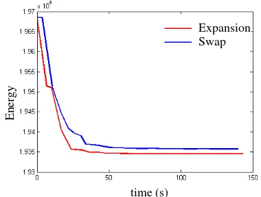
The quantitative characteristics of theα-expansion and theα−β swap algorithms are summarized in Table 1. In order to demon-strate the behavior of the energy function during the optimiza-tion process, its values are plotted with respect to the time (in seconds) for the two minimization algorithms,α-expansion and α−βswap. The results forλ= 0.5 andT= 0 are shown in Figure 10.
Expansion Swap
time (s)
Ener
gy
Figure 10. Energy minimization function with respect to time (in seconds) forα-expansion andα−βswap algorithms (T= 0 and λ= 0.5).
Regarding the obtained results, where we investigated the influ-ence of the balancing parameterλand the truncation constantT on method’s performance by running two energy minimization algorithms,α-expansion andα-βswap, we can conclude that:
• By finding a good trade-off between the data term and reg-ularization term in Equation (9) we can improve the visual quality of our textured model. Some lighting variations are still present, especially on the buildings with sophisticated design (the facades and roofs contain many features).
• Varying only the balancing parameterλis not enough to get a satisfying visual appearance of the model. Additionally using a truncation constantT helps to preserve the bound-aries between regions with significant texture variations. It should be mentioned that in previous work the truncation constantTwas not taken into account.
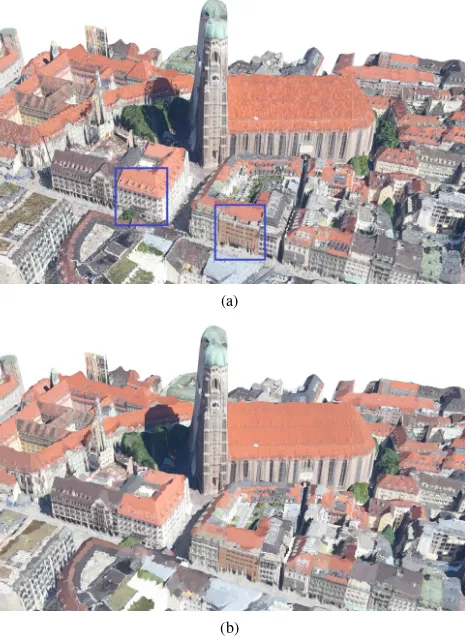
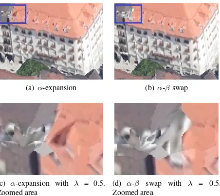
(a)α-expansion (b)α-βswap
(c) α-expansion with λ = 0.5. Zoomed area
(d) α-β swap with λ = 0.5. Zoomed area
Figure 11. Comparison study between α-expansion and α-β swap performances (λ= 0.5).
Figure 11a - 11b. Here we examine the region highlighted with blue rectangles. The magnified vesions are presented in Figure 11c and 11d. From this example we can see that α-expansion found a closer to optimal solution for textur-ing the red roof than theα-βswap. This is consistent with the evolution of the energy function with respect to the time for bothα-expansion andα−βswap algorithm, as demon-strated in Figure 10. The values of the energy function found by running theα-expansion algorithm are lower than for the α−βswap algorithm. Additionally, from the results pre-sented in Table 1 we can see that the amount of time theα -expansion algorithm needs to find a local minimum is less than for theα-βswap. This can be explained by the fact that in one cycle the swap algorithm takes|L|2iterations, and for the expansion it is|L|iterations in one cycle.
For the real-world dataset, which we used in this work for cre-ation a textured 3D scene of the city center of Munich, there is no public ground truth data available. Additionally, every other author who is doing similar work uses/used his private dataset. Thus, we can not compare the performance of our method against theirs. This is one of the problems in the field of texturing 3D models. It would be probably the most important work in the future to provide a public dataset for making all the algorithms comparable.
A limitation of the presented approach can be a significant dif-ference in the size of adjacent triangles in a model, which in-fluences the texture assignment. In the given data (obtained by aerial image matching) this is the case when one triangle belongs to the building’s facade and its neighbor to the roof. The trian-gles belonging to the facades are bigger compared to the triantrian-gles on the roofs due to a sparser point cloud in these regions. This means that the projection of big triangles onto 2D image space could cover many pixels with very different colors. As a result the average RGB color of these triangles could be significant dif-ferent from the average RGB color of the neighboring triangles (which are on the roofs), even if the area close to the common edge between triangles looks similar. Consequently, the texture assignment is penalized, which is incorrect.
5. SUMMARY AND OUTLOOK
Our results confirm that a Markov Random Field energy mini-mization approach enables us to perform fully automatic textur-ing of large-scale 3D models from high-resolution photographic images minimizing lighting variations across the areas where im-ages are overlapping. In contradiction to previous approaches, the use of Markov Random Fields energy minimization allows to keep the resolution of the produced texture, which is essentially the same as that of the original views. That means the detail-rich information which is contained in high-resolution photographic images, is completely transmitted to the reconstructed models. Our technique is based on the techniques presented in (Allene et al., 2008), (Gal et al., 2010) and (Lempitsky and Ivanov, 2007) with a few modifications for the energy function: The first term, which measures the visual details of each face, is computed as a combination of a number of visible pixels of a given face and the angle between the face’s normal and the looking vector of the camera. The second term, which measures the color continuity between adjacent faces, is computed as difference of the average RGB color per triangle. Moreover, in previous works the prob-lem was addressed only to texture small test sites. We extended our multi-view texturing approach for large-scale scenes. There are mainly two parameters in the Markov Random Field energy minimization which influence the results: The trunca-tion constantT and the balancing parameterλ. Both of them should be set, because using only the balancing parameterλis not enough to get a satisfying visual appearance of the model. This finding became one of the main benefits in this work. By choosing appropriate values of these parameters we showed that a close to optimal seam placement can be achieved. As possible extension to this research additional post-processing steps can be applied to perform further color corrections.
REFERENCES
Alj, Y., Boisson, G., Bordes, P., Pressigout, M. and Morin, L., 2012. Multi-texturing 3d models: How to choose the best texture? In: 3D Imaging (IC3D), 2012 International Conference on, IEEE, pp. 1–8.
Allene, C., Pons, J.-P. and Keriven, R., 2008. Seamless image-based texture atlases using multi-band blending. In: Pattern Recognition, 2008. ICPR 2008. 19th International Conference on, IEEE, pp. 1–4.
Baumberg, A., 2002. Blending images for texturing 3d models. In: BMVC, Vol. 3, p. 5.
Blake A., Kohli P., R. C., 2011. Markov random fields for vision and image processing. MIT Press.
Boykov, Y. and Kolmogorov, V., 2004. An experimental compar-ison of min-cut/max-flow algorithms for energy minimization in vision. Pattern Analysis and Machine Intelligence, IEEE Trans-actions on 26(9), pp. 1124–1137.
Boykov, Y., Veksler, O. and Zabih, R., 2001. Fast approximate energy minimization via graph cuts. Pattern Analysis and Ma-chine Intelligence, IEEE Transactions on 23(11), pp. 1222–1239.
Debevec, P. E., Taylor, C. J. and Malik, J., 1996. Modeling and rendering architecture from photographs: A hybrid geometry-and image-based approach. In: Proceedings of the 23rd annual con-ference on Computer graphics and interactive techniques, ACM, pp. 11–20.
Frueh, C., Sammon, R. and Zakhor, A., 2004. Automated tex-ture mapping of 3d city models with oblique aerial imagery. In: 3D Data Processing, Visualization and Transmission, 2004. 3DPVT 2004. Proceedings. 2nd International Symposium on, IEEE, pp. 396–403.
Gal, R., Wexler, Y., Ofek, E., Hoppe, H. and Cohen-Or, D., 2010. Seamless montage for texturing models. In: Computer Graphics Forum, Vol. 29number 2, Wiley Online Library, pp. 479–486.
Hoegner, L. and Stilla, U., 2009. Thermal leakage detection on building facades using infrared textures generated by mobile mapping. In: Urban Remote Sensing Event, 2009 Joint, IEEE, pp. 1–6.
Iwaszczuk, D., Helmholz, P., Belton, D. and Stilla, U., 2013. Model-to registration and automatic texture mapping using a video sequence taken by a mini uav. ISPRS-International Archives of the Photogrammetry, Remote Sensing and Spatial In-formation Sciences 1(1), pp. 151–156.
Iwaszczuk, D., Hoegner, L. and Stilla, U., 2011. Matching of 3d building models with ir images for texture extraction. In: Urban Remote Sensing Event (JURSE), 2011 Joint, IEEE, pp. 25–28.
Kolecki, J., Iwaszczuk, D. and Stilla, U., 2010. Calibration of an ir camera system for automatic texturing of 3d building models by direct geo-referenced images. Proceedings of Eurocow.
Kolmogorov, V. and Rother, C., 2006. Comparison of energy minimization algorithms for highly connected graphs. In: Com-puter Vision–ECCV 2006, Springer, pp. 1–15.
Kolmogorov, V. and Zabin, R., 2004. What energy functions can be minimized via graph cuts? Pattern Analysis and Machine Intelligence, IEEE Transactions on 26(2), pp. 147–159.
Kurz, F., M¨uller, R., Stephani, M., Reinartz, P. and Schroeder, M., 2007. Calibration of a wide-angle digital camera system for near real time scenarios. In: ISPRS Hannover Workshop, pp. 1682– 1777.
Kuschk, G., 2013. Large scale urban reconstruction from remote sensing imagery. International Archives of the Photogrammetry, Remote Sensing and Spatial Information Sciences 5, pp. W1.
Lempitsky, V. and Ivanov, D., 2007. Seamless mosaicing of image-based texture maps. In: Computer Vision and Pattern Recognition, 2007. CVPR’07. IEEE Conference on, IEEE, pp. 1– 6.
Pelagottia, A., Del Mastio, A., Uccheddu, F. and Remondino, F., 2009. Automated multispectral texture mapping of 3d models. EUSIPCO 2009.
Rocchini, C., Cignoni, P., Montani, C. and Scopigno, R., 1999. Multiple textures stitching and blending on 3d objects. In: Pro-ceedings of the 10th Eurographics conference on Rendering, Eu-rographics Association, pp. 119–130.
Szeliski, R., Zabih, R., Scharstein, D., Veksler, O., Kolmogorov, V., Agarwala, A., Tappen, M. and Rother, C., 2006. A compar-ative study of energy minimization methods for markov random fields. In: Computer Vision–ECCV 2006, Springer, pp. 16–29.
Veksler, O., 2007. Graph cut based optimization for mrfs with truncated convex priors. In: Computer Vision and Pattern Recog-nition, 2007. CVPR’07. IEEE Conference on, IEEE, pp. 1–8.