INTERESTING SPATIO-TEMPORAL REGION DISCOVERY COMPUTATIONS OVER
GPU AND MAPREDUCE PLATFORMS
Michael McDermotta,∗, Sushil K. Prasadb, Shashi Shekharc, and Xun Zhoud a
Department of Computer Science, Georgia State University, USA - [email protected] bDepartment of Computer Science, Georgia State University, USA - [email protected] c
Department of Computer Science, University of Minnesota, USA - [email protected] dDepartment of Management Sciences, University of Iowa, USA - [email protected]
KEY WORDS:GPU, MapReduce, Hadoop, Parallelism, GIS, Spatial, Spatio-Temporal, Data Mining
ABSTRACT:
Discovery of interesting paths and regions in spatio-temporal data sets is important to many fields such as the earth and atmospheric sciences, GIS, public safety and public health both as a goal and as a preliminary step in a larger series of computations. This discovery is usually an exhaustive procedure that quickly becomes extremely time consuming to perform using traditional paradigms and hardware and given the rapidly growing sizes of today’s data sets is quickly outpacing the speed at which computational capacity is growing. In our previous work (Prasad et al., 2013a) we achieved a 50 times speedup over sequential using a single GPU. We were able to achieve near linear speedup over this result on interesting path discovery by using Apache Hadoop to distribute the workload across multiple GPU nodes. Leveraging the parallel architecture of GPUs we were able to drastically reduce the computation time of a 3-dimensional spatio-temporal interest region search on a single tile of normalized difference vegetative index for Saudi Arabia. We were further able to see an almost linear speedup in compute performance by distributing this workload across several GPUs with a simple MapReduce model. This increases the speed of processing 10 fold over the comparable sequential while simultaneously increasing the amount of data being processed by 384 fold. This allowed us to process the entirety of the selected data set instead of a constrained window.
1 INTRODUCTION
Interesting path and interesting spatio-temporal region discovery are important filtering steps in many domains such as earth and atmospheric sciences, GIS, public safety, public health and other fields which deal with identifying and analyzing spatial data that change over time. These are typically computationally expen-sive steps and can take hours to days to complete. For instance filtering non-interesting paths and regions is of particular inter-est when predicting weather patterns, designing accurate ecolog-ical models of climate shift and tracking ecotone1boundaries and changes. Tracking these boundaries is a good way to study de-sertification, deforestation, erosion and other shifts in geographic areas which is of particular interest to GIS and environmental sci-entists.
Finding interesting paths and spatio-temporal regions are exhaus-tive operations. The reason for this is that the path or region does not necessarily have a clearly defined limit. In other words the interesting path or region could be as small as one item or as large as the whole data set (Zhou et al., 2011, Zhou et al., 2013). This leads to the less obvious, but important, consideration which is that any given interesting region or path may be contained in inside another larger region or path and this must be addressed somehow (Zhou et al., 2011, Zhou et al., 2013).
Data growth is also quickly outpacing our computational and management abilities on traditional hardware and algorithm im-plementations. More efficient ways of filtering and processing this data are important to develop in order to complete the com-putation in a reasonable time frame.
Parallel and distributed designs and implementations of these more efficient algorithms are also therefore becoming increasingly
im-∗Corresponding author
1
Ecotones are transitions between different ecologies such as the boundary be-tween forest and grasslands (Zhou et al., 2011).
portant. Currently these sorts of big data calculations are limited to large clusters and supercomputers which are capable of pro-cessing the large volumes of data. Supercomputing environments are however expensive in time and effort to setup, manage and use. A much more accessible and economic approach is to equip a workstation with one or more inexpensive yet high performance GPU’s which would allow rapid testing and deployment of new algorithms to solve problems in these domains. GPU hardware is economical both in terms of price to performance and in terms of power consumption to compute ability.
This paper’s contributions are :
• To leverage GPU hardware to speed up discover of spatio-temporal regions of interest from anO(M2
N2
T2
) compu-tation to anO(M N T2
)computation.
• To use a MapReduce model to distribute discovery of spatio-temporal regions of interest across multiple GPU devices which provides linear speedup with respect to the number of GPU devices used.
• To use Apache Hadoop to distribute interesting path discov-ery across multiple GPU compute nodes which provides a linear speedup over our previous work with respect to the number of nodes used.
• Sequential algorithms have problems processing large sizes of data (eg: the4800×4800map tiles discussed in Section 5) and have to limit computation to a smaller subset (eg: 200×300) in order to complete computation (Zhou et al., 2013). We have increased the size of the data that can be processed to the full map tile while simultaneously increas-ing performance for similar window sizes.
related works. In Section 4 we give an overview of the most im-portant GPU considerations for this work and give a general de-sign overview of our implementations of Hadoop+GPU subpath discovery, GPU Region discovery and GPU MapReduce ST-Region Discovery. In Section 5 we discuss the hardware environ-ment used for our experienviron-ments. Section 6 shows our experimen-tal results for Hadoop+GPU subpath discovery, GPU ST-Region discovery and GPU MapReduce ST-Region Discovery. Section 7 concludes the paper and gives some of our future research goals.
2 PROBLEM DESCRIPTION
In this work we are concerned with processing the large volumes of spatio-temporal data produced by remote sensing technologies frequently used in the study of climatology, oceanography, and geology. This data is generally stored in either vector or raster form. For our purposes we were interested in detecting paths and spatio-temporal regions of rapid change in normalized differ-ence vegetative index data (NDVI) sets which are stored in raster image form2. These are frequently pre-processing steps used to limit the data being considered by much more costly computa-tions and are also used to reveal interesting information in their own right. These problems are themselves computationally ex-pensive as they must exhaustively consider the entire data set.
2.1 Path Discovery
Discovering interesting paths is the problem of discovering one dimensional longitudinal subpaths in a given raster data set that show increases (or decreases) in average NDVI value greater than a threshold value.
Path Discovery
Given:
• An array of elementsS • A thresholdθ
• A score functionF Find:
• All subpathss∈SwhereF(s)> θ
The determination of interestingness is described by Equation 1,
F(s) = Average value of unit subpath > θ
Average value of all unit subpaths > θ (1)
as in (Zhou et al., 2011, Prasad et al., 2013a).
Naively this test is trivial to implement but is computationally expensive with a cost ofO(N2
M)for anN×Mtile of data. As we have to examineN−1subpaths for everyN items and we must do thisM times. This quickly becomes problematic with today’s large data sets.
(Zhou et al., 2011) provides an SEPalgorithm which reduces computation by an order of magnitude over naive implementa-tions through the construction of a lookup table inO(N)time. This lookup table reduces anO(N) scan operation to anO(1) lookup, reducing the overall complexity toO(N) +O(N2).
The SEP algorithm has three phases:
1. Build the lookup table
2. Discover all interesting sub paths
2
For more information on NDVI and these datasets see Section 5.
3. Eliminate paths which are subsets of longer paths
The lookup table is a simple columnar prefix sum of the data in question. This can be done inO(M N)time for spatial data of dimensionM xN(Zhou et al., 2011, Prasad et al., 2013a). Each column for the purposes of the discovery is assumed independent.
The discovery phase then uses the lookup table to find subpaths that pass the interestingness test. Longitudinal subpaths are pre-ferred due to their being more likely to span ecotone boundaries (Zhou et al., 2011). This test is performed for each possible sub-path in a given column and for each column of data starting at the largest possible subpath and examining each smaller subpath in turn until one is found that is interesting.
The elimination phase examines all discovered sub-paths and elim-inates any that are completely enclosed inside a longer subpath.
2.2 Spatio-temporal Region Discovery
Discovering interesting spatio-temporal subregions is the prob-lem of finding a two dimensional subregion that exhibits average change in NDVI value greater than a threshold value for a given interval of time.
ST-Region Discovery
Given
• A set ofRofM xNregions organized by time • A time interval to considerT
• A thresholdΘ
• A score functionF Find
• All sub-regionsrthat are interesting
The interestingness test is described by Equation 2.
F(S) =Average change in value f or the subregion
time interval (2)
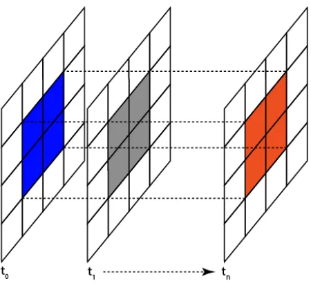
As in (Zhou et al., 2013) this average change in value is defined as the value of the subregion at the beginning of the time interval minus the value of subregion at the end of the interval divided by the value of the beginning subregion. This is a measure of the average decrease in NDVI value. These beginning and ending values are determined by summing all the values in the subregion being considered. This must be done for both the beginning and the end of the interval being considered. This is illustrated in Fig-ure 1 where the subregion at the beginning of the time interval is shown in blue and the corresponding subregion at the end of the time interval is shown in orange. The gray shaded region repre-sents one of the possibly many intermediate subregions contained in the spatio-temporal volume being considered. For Figure 1 the time interval being considered isnas it spansn+ 1parent re-gions.
Naively this is also trivial to implement with the computational complexity increasing toO(M4N4T2)in the worst case. This is due to the need to exhaustively examine all possible spatio-temporal volumes. For small windows this computation time may be acceptable however in today’s big data environment the time needed to perform this operation quickly becomes unacceptable asM,NandTbecome large.
Figure 1. Subregion Discovery fort0...tn
the worst case complexity to O(M2
N2
T2
)by pre-computing a lookup table. This lookup table takesO(M N)time andO(M N) space in exchange for significantly reducing overall time com-plexity in a similar way to the SEP algorithm.
This algorithm also has three phases:
1. Build the lookup table
2. Discover all interesting subregions
3. Eliminate all subregions which are within larger regions
The discovery phase is also similarly scaled up in dimensions. The use of the lookup table is particularly important as it replaces anO(N M T)scan for anO(1)lookup. The elimination phase is also similarly scaled up and in this phase all PCW embedded in larger PCW are removed from results.
3 PREVIOUS AND RELATED WORK
3.1 Previous Work
In our previous work on interesting path discovery, the GPU im-plementation is straightforward due to the data independent na-ture of the problem (Prasad et al., 2013a). The lookup table is embarrassingly parallel to implement by launching a thread for everyn∈N. By coalescing memory access the GPU is used ef-ficiently to compute this scan very quickly. It should be noted that this is not truly a parallel scan but simply many smaller sequen-tial scans launched in parallel. Due to the size of the data used for this work the performance impact was deemed to be negligible.
The subpath discovery is sped up significantly due also to the data independent nature of the problem. A worse caseO(N2
M) problem is reduced in theoretical complexity toO(N M)through parallelization on the GPU (Prasad et al., 2013a).
The elimination step here was accomplished two ways; implic-itly and explicimplic-itly. Implicit elimination allows larger subpaths to overwrite smaller ones when the data is visualized. Explicit elim-ination programatically removes smaller subpaths that are com-pletely embedded in larger subpaths. The complexity of explicit elimination is the same as with discovery (Prasad et al., 2013a).
Overall this resulted in a good speedup and the ability to process a single image in the data set in roughly 30ms. We were able to
process the entire data set quickly enough to generate real-time visualizations of the algorithm’s output on a single GPU (Prasad et al., 2013b, Prasad et al., 2013a). We use this data set and GPU implementation in Section 4.1.
3.2 Related Work
MapReduce is a high level data centric model of distributed com-puting that only requires two main phases; the map phase to dis-tribute data and the reduce phase to perform computation and re-turn results.
There are currently few related works dealing with MapReduce and GPU. The first is Mars, a GPU MapReduce framework im-plemented on GPUs in C/C++ and Cuda (He et al., 2008). This uses a simplified version of MapReduce which only has two phases, map and reduce. The second is GPMR, a GPU MapReduce li-brary geared towards GPU clusters with scalability as a specific concern (Stuart and Owens, 2011). Self contained and extensi-ble, the GPU is still exposed to the user in contrast to Mars which sought to obfuscate the GPU behind its own MapReduce inter-face. The third, StreamMR, is a GPU MapReduce framework based on OpenCL and designed for clusters of AMD GPUs (El-teir et al., 2011).
There are two main works that deal specifically with MapRe-duce and spatial data: Hadoop and HadoopGIS. Spatial-Hadoop is an extension of Spatial-Hadoop that provides access to spa-cial primitives and common spatial operations (Eldawy, 2014). HadoopGIS is a spatial data query system for performing spatial queries in Hadoop (Aji et al., 2013). However, neither Spatial-Hadoop nor Spatial-HadoopGIS have built-in support for GPU integra-tion currently.
4 DESIGN AND IMPLEMENTATION DETAILS
In order to achieve the best performance from the GPU hardware some general guidelines and best practices must be followed.
CUDA General Guidelines
• Minimize branching
• Minimize global memory access
• Maximize global memory bandwidth utilization
Minimizing branching has to do with the GPU being a single in-struction multiple data (SIMD) architecture. Threads in a block are grouped together into warps of up to 32 threads with threads within a warp ideally executing the same instruction. When there is branching within a warp there is the potential to halve the per-formance of the warp. With enough branching this can reduce performance to near sequential time.
Minimizing global memory access and maximizing global mem-ory bandwidth utilization are closely related. Global memmem-ory, the large memory measured in gigabytes on the GPU device, has very slow access time compared to the local thread memory and shared block memory which are much smaller. When accessing global memory, for maximum performance, it must be accessed in a thread aligned way. This means that threads in the same warp access contiguous portions of global memory in order to speed up access and maximize throughput (NVIDIA, 2013).
4.1 GPU+Hadoop Path Discovery
Using the single GPU implementation from our previous work (Prasad et al., 2013a), the Hadoop implementation is fairly straight-forward. At the high level:
1. Raw raster data is read into a sequence file on and saved on the HDFS.
2. Values are mapped from the sequence file.
3. GPU computation is performed on compute nodes in the re-duce phase.
GPU kernels were written in CUDA and then launched by Hadoop using the JCUDA3Java bindings library. This allowed quick de-ployment to Hadoop once the GPU code had been developed.
This also means that care must be taken in the map phase so that the data is not subdivided incorrectly. We used a sequence file to guarantee that this did not happen. This also allowed us to keep the data in a binary format (White, 2009). Using the sequence file allowed avoidance of the small files problem as we were able to read in all the relatively small raster data files and combine them into one large file ofkey, valuepairs. For simplicity each raster data file was read in as a single value in the sequence file.
The small file problem stems from how the HDFS maps files. Each file in HDFS uses at least one HDFS block. For files larger than this block size this is generally not an issue. When files are smaller than the block size then space in the HDFS is wasted. This can potentially result in decreased performance of the HDFS as a whole by increasing file read and write (White, 2009).
4.2 GPU Spatio-temporal Region Discovery
The previous paradigm for building the looking table, while sple, is comparatively inefficient. A better strategy is a GPU im-plementation of parallel prefix sum due to the size of the data set. This algorithm is adapted from the segmented sums algorithm of (Nguyen, 2007) and is sketched briefly in Algorithm 1. This al-gorithm suffers from the limitation that it cannot perform a prefix sum on an array larger than the maximum threads allowed in a block. In order to overcome this limitation a segmented sum is used. The last element of each prefix summed block of threads is used to populate a new array which is then prefix summed with the same algorithm and limitations. This is done as a reduction tree until a single block of threads can process the array. These values are then back-propagated up through the reduction tree in parallel. This back-propagation step can be seen in Figure 2.
Algorithm 1: High Level View Of Scan (Nguyen, 2007)
1: procedureSCAN(data) 2: perform in parallel upsweep 3: perform in parallel downsweep
4: ifblock count6= 0then
5: lastItem←blockDim−1
6: ifthreadId==lastItemthen 7: last[blockId]←item[threadId]
8: end if
9: end if
10: end procedure
This scan is complex and requires multiple kernel invocations but it leverages the strengths of the GPU extremely well. The overall complexity for construction of the table isO(N logM).
3
For more information seehttp://www.jcuda.org
Figure 2. Illustration of segmented scan propagation (Nguyen, 2007)
The PCW algorithm is straightforward to parallelize due to the relative independence of each subregion being considered. It is performed in parallel with a thread for each starting position. This reduces the complexity to a theoreticalO(M N T2
)computation whenM N threads are used. AnO(1)lookup is performed in order to retrieve the subregion values needed for Equation 2.
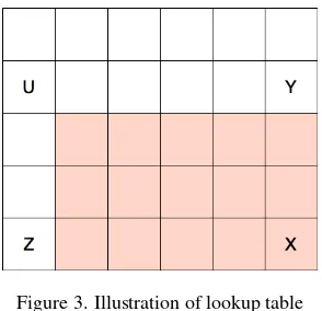
This lookup is described by Equation 3.
X
subregion value=XX−XY−XZ+XU (3)
Where X, Y, Z, and U are the prefix sums at the locations shown in Figure 3 and we want the value associated with the subregion described by the shaded portion of Figure 3.
Figure 3. Illustration of lookup table
This is an efficient operation and widely used in many computer graphics domains (Crow, 1984, Zhou et al., 2013).
The implementation details of the algorithm require significant re-engineering in order to reduce branching to a minimum, max-imize memory bandwidth, coalesce memory access and ensure that blocks of threads never consider areas that are outside the dimensions of the data set. The high level algorithm sketch for a thread block is shown in Algorithm 2.
Each block of threads retrieves start locations and then iteratively retrieves possible end locations and performs this discovery test. When the discovery test is finished the block gets the next block sized subset of end locations.
Algorithm 2: High Level Block based discovery
1: procedureDISCOVERY(region)
2: copy global region U,X,Y,Z to shared U,X,Y,Z
3: region sum =PX−PY −PZ+PU 4: do interestingness test (Equation 2) 5: copy results to global memory
6: end procedure
4.3 Multiple-GPU MapReduce Spatio-Temporal Region Dis-covery
The multiple GPU MapReduce model is straightforward due to the overall design of the GPU implementation being itself a Map-Reduce model. Each time interval calculation is also independent for the interestingness test and easily maps to a distinct GPU. For instance the calculations needed for intervalt0...tiare
indepen-dent of those needed for intervalt0...tj. Each GPU also has its
own unique device ID, making it easy to iterate through the time intervals and assign an interval to a specific device. It is straight-forward to do this assignment, computation, and memory trans-fer asynchronously (NVIDIA, 2012), allowing the devices to run independently of each other and the CPU. As each device fin-ishes a time interval it reduces the output back to the CPU asyn-chronously then it immediately starts on the next interval it has been mapped.
Algorithm 3: High Level View of Map Reduce for Multi-GPU
1: fori= 0→intervalCountdo
2: id←i%deviceCount 3: map interval[i] to device[id] 4: forj=intervalCount→i+ 1do
5: map interval[j] to device[id] 6: computeP CW()
7: end for
8: reduce output to CPU 9: end for
5 DATA AND HARDWARE ENVIRONMENT
The datasets used are normalized difference vegetative index data (NDVI); a measure of vegetative density. NDVI is computed by measuring reflectance of specific wavelengths of light off the surface of the earth through remote sensing (Weier and Herring, 2000).
5.1 GPU+Hadoop Path Discovery
GPU+Hadoop Path discovery was performed using a heteroge-neous cluster environment and the same data set as in our previ-ous work. This cluster consists of several nodes equipped with NVIDIA GTX 480 and NVIDIA Tesla C2075 GPUs. The data set used is the Global Inventory Modeling and Mapping Studies (GIMMS) data set which consists of 20 years of NDVI resulting in 611 images of Africa of size1152×1152(Tucker and Brown, 2004). This data set was used in order to do a fair comparison be-tween the GPU, Hadoop with GPU, and sequential environments. Nodes are equiped with memory ranging from 8GB to 64GB of memory and either dual Intel Xeon Quad Core 5410 or dual Intel Xeon E5-2650 CPUs.
5.2 Spatio-Temporal Region discovery
Spatio-Temporal Region discovery was performed using NVIDIA Tesla k20 GPUs. The data set used was a subset of NDVI data
taken from the Land Processes Distributed Active Archive Cen-ter (LPDAAC) and consists of 12 years, 2000 through 2012, of 4800×4800NDVI data selected from the NASA MODIS project (NASA and USGS, 2015). As stated in (Zhou et al., 2013) the se-quential discovery algorithm was limited to a small subsection of this data set (200×300), however, on the GPU we processed the entire4800×4800map tile. MapReduce was implemented on a single compute node that housed four Tesla k20 GPUs. This node is equipped with 64GB of memory and dual Intel Xeon E5-2650 CPUs.
6 EXPERIMENTAL RESULTS
Initial results are very promising and significant performance in-creases were achieved by porting to GPU and Multi-GPU envi-ronments.
6.1 GPU+Hadoop Path Discovery
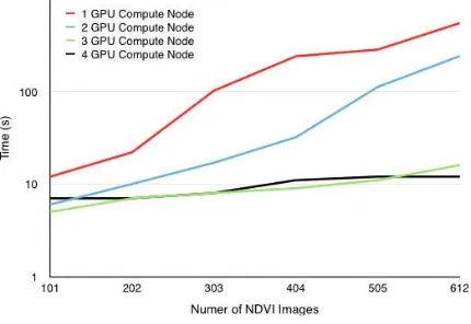
The Hadoop implementation resulted in a nearly linear speedup with the addition of more nodes as can be seen in Figure 4 but also made realizing real-time visualization impossible. There are di-minishing returns as more nodes are added. It is expected that this is because of the data size being relatively small at only roughly 300MB for the entire 611 NDVI images.
Figure 4. Path Discovery Hadoop Scaling
6.2 Spatio-Temporal Region Discovery
Compute speeds increased 50 fold over naive sequential, which was expected due to performance increases seen for the sequen-tial SEP algorithm. Compute speeds increased 10 fold compared to SEP algorithm. These speedups do not at first seem impressive however it must be kept in mind that the largest PCW processed sequentially in (Zhou et al., 2013) was a50×50subregion on a very limited subwindow of200×300; no such artificial con-straint on window size was enforced on the GPU implementation and we processed the entire raster tile exhaustively.
This means the realized speedup is comparing computation on a 200×300window to computation on a4800×4800window. In other words we realized a good speedup and simultaneously were able to increase the maximum potential window size by 384 fold.
Figure 5. ST-Region GPU MapReduce timing with varying win-dow dimension (time intervalT = 10)
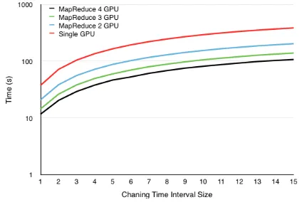
Figure 6. ST-Region GPU MapReduce with varying Time inter-val size (fixed dimension =75×75)
Holding the PCW dimensions fixed at75×75we can see the effects here of varying the time interval in Figure 6.
Both plots demonstrate how scaling is affected by varying di-mensions. Adding GPUs has diminishing returns for small query sizes, however the scaling approaches linear for the larger queries. This reduces total time taken by a factor equal to the number of GPUs used.
7 CONCLUSION AND FUTURE WORK
This work explores an implementation of the SEP and PCW al-gorithms from (Zhou et al., 2011, Zhou et al., 2013) that clearly show an increase not just in execution time but in the amount of data that can be processed. While valuable in its own right this is also a valuable consideration for what may be a preprocessing step for a much larger and more intensive computational model. Offloading this processing onto the GPU, while more time con-suming in the development phase, is a viable technique to speed up these calculations. This will become increasingly more im-portant to achieve as big data considerations continue to become more and more important to address.
Future works include a GPU and GPU+MapReduce model for the elimination phase in the PCW algorithm as well as processing multiple tiles.
REFERENCES
Aji, A., Wang, F., Vo, H., Lee, R., Liu, Q., Zhang, X. and Saltz, J., 2013. Hadoop gis: A high performance spatial data warehousing
system over mapreduce. Proc. VLDB Endow. 6(11), pp. 1009– 1020.
Crow, F. C., 1984. Summed-area tables for texture mapping. SIG-GRAPH Comput. Graph. 18(3), pp. 207–212.
Eldawy, A., 2014. Spatialhadoop: Towards flexible and scal-able spatial processing using mapreduce. In: Proceedings of the 2014 SIGMOD PhD Symposium, SIGMOD’14 PhD Sym-posium, ACM, New York, NY, USA, pp. 46–50.
Elteir, M., Lin, H., Feng, W.-c. and Scogland, T., 2011. Streammr: An optimized mapreduce framework for amd gpus. In: Proceedings of the 2011 IEEE 17th International Conference on Parallel and Distributed Systems, ICPADS ’11, IEEE Com-puter Society, Washington, DC, USA, pp. 364–371.
He, B., Fang, W., Luo, Q., Govindaraju, N. K. and Wang, T., 2008. Mars: A mapreduce framework on graphics processors. In: Proceedings of the 17th International Conference on Paral-lel Architectures and Compilation Techniques, PACT ’08, ACM, New York, NY, USA, pp. 260–269.
NASA and USGS, 2015. http://lpdaac.usgs.gov/ products/modis_products_table/mod13q1.
Nguyen, H., 2007. Gpu Gems 3. First edn, Addison-Wesley Professional.
NVIDIA, 2012. http://devblogs.nvidia.com/ parallelforall/how-overlap-data-transfers-cuda-cc/.
NVIDIA, 2013. http://devblogs.nvidia.com/
parallelforall/how-access-global-memory-efficiently-cuda-c-kernels/.
Prasad, S. K., Shekhar, S., McDermott, M., Zhou, X., Evans, M. and Puri, S., 2013a. GPGPU-accelerated interesting inter-val discovery and other computations on geospatial datasets: A summary of results. In: Proceedings of the 2Nd ACM SIGSPA-TIAL International Workshop on Analytics for Big Geospatial Data, BigSpatial ’13, ACM, New York, NY, USA, pp. 65–72.
Prasad, S., Shekhar, S., He, X., Puri, S., McDermott, M., Zhou, X. and Evans, M., 2013b. Gpgpu-based data structures and al-gorithms for geospatial computation a summary of results and future roadmap (position paper). Proceedings of The All Hands Meeting of the NSF CyberGIS project, Seattle.
Stuart, J. A. and Owens, J. D., 2011. Multi-gpu mapreduce on gpu clusters. In: Proceedings of the 2011 IEEE International Parallel & Distributed Processing Symposium, IPDPS ’11, IEEE Computer Society, Washington, DC, USA, pp. 1068–1079.
Tucker, C.J., J. P. and Brown, M., 2004. Global Inventory Mod-eling and Mapping Studies, NA94apr15b.n11-VIg, 2.0. Global Land Cover Facility, University of Maryland, College Park, Maryland.
Weier, J. and Herring, D., 2000. Measuring vegetation (ndvi & evi). http://earthobservatory.nasa.gov/Features/ MeasuringVegetation/.
White, T., 2009. Hadoop: The Definitive Guide. 1st edn, O’Reilly Media, Inc.