ESTIMATION OF ANNUAL AVERAGE SOIL LOSS, BASED ON RUSLE MODEL IN
KALLAR WATERSHED, BHAVANI BASIN, TAMIL NADU, INDIA
S. Abdul Rahaman a, *, S. Aruchamy b, R. Jegankumar c, S. Abdul Ajeez d
a Research Fellow, Dept. of Geography, Bharathidasan University, Tiruchirappalli, Tamil Nadu, India.- [email protected] b Professor, Dept. of Geography, Bharathidasan University, Tiruchirappalli, Tamil Nadu, India. [email protected]
c Assistant Professor, Dept. of Geography, Bharathidasan University, Tiruchirappalli, Tamil Nadu, India. - [email protected] d Team Leader, Research and Development, Lumina Datamatics, Chennai, Tamil Nadu, India - [email protected]
KEY WORDS: Soil Erosion, Soil Loss, Erosivity, Erodability, Erosion Risk, RUSLE, Remote Sensing and GIS
ABSTRACT:
Soil erosion is a widespread environmental challenge faced in Kallar watershed nowadays. Erosion is defined as the movement of soil by water and wind, and it occurs in Kallar watershed under a wide range of land uses. Erosion by water can be dramatic during storm events, resulting in wash-outs and gullies. It can also be insidious, occurring as sheet and rill erosion during heavy rains. Most of the soil lost by water erosion is by the processes of sheet and rill erosion. Land degradation and subsequent soil erosion and sedimentation play a significant role in impairing water resources within sub watersheds, watersheds and basins. Using conventional methods to assess soil erosion risk is expensive and time consuming. A comprehensive methodology that integrates Remote sensing and Geographic Information Systems (GIS), coupled with the use of an empirical model (Revised Universal Soil Loss Equation- RUSLE) to assess risk, can identify and assess soil erosion potential and estimate the value of soil loss. GIS data layers including, rainfall erosivity (R), soil erodability (K), slope length and steepness (LS), cover management (C) and conservation practice (P) factors were computed to determine their effects on average annual soil loss in the study area. The final map of annual soil erosion shows a maximum soil loss of 398.58 t/h-1/y-1. Based on the result soil erosion was classified in to soil erosion severity map with five classes, very low, low, moderate, high and critical respectively. Further RUSLE factors has been broken into two categories, soil erosion susceptibility (A=RKLS), and soil erosion hazard (A=RKLSCP) have been computed. It is understood that functions of C and P are factors that can be controlled and thus can greatly reduce soil loss through management and conservational measures.
* Corresponding author
1. INTRODUCTION
“Erosion is a process of detachment and transport of soil particles by erosive agents - Ellison, (1944)”. Detachment of individual particles from soil aggregates, Transport of particles by erosive agents by water or wind. Particles are eventually deposited to form new soils or to fill lake and reservoir.
Worldwide, each year, about 75 billion tons of soil is eroded from the land, a rate that is about 13-40 times as fast as the natural rate of erosion, Zuazo et al. (2009). Asia has the highest soil erosion rate of 74 ton/acre/ year, El-Swaify S.A., (1997). In India, the soil erosion is more severe in the Himalayan ranges, Northeastern states, and the Western Ghats, together constitute 45% (130M ha) of the total geographic area, which is affected by serious soil erosion through ravines, gullies, shifting cultivation, cultivated wastelands, sandy areas, deserts, and water logging. Among this 93.68M ha of land is influenced by hydrologically controlled soil erosion (Narayan and Babu 1983; Anon 2008, 2009; Singh et al. 1992; Pandey et al.2007). In recent years, as part of environment and land degradation assessment policy for sustainable agriculture and development, soil erosion is increasingly being recognized as a hazard which is more serious in mountain areas (Millward and Mersey, 1999; Angima et al., 2003; Jasrotia and Singh, 2006; Dabral et al., 2008; Sharma, 2010). Soil erosion causes siltation of reservoirs, which ultimately reduces the life of the project and affects generation of hydroelectric power (Jasmin and Ravichandran, 2006).
Erosion models can be used as predictive tools for assessing soil loss and soil erosion risk for conservation planning (Poppet al. 2000). A quantitative assessment is needed to infer the extent and magnitude of soil erosion problems so that effective management strategies can be resorted to. But, the complexity of the variables makes precise estimation or prediction of erosion is difficult. The latest advances in spatial information technology have improved the existing methods and have provided efficient methods of monitoring, analysis and management of earth resources. Digital elevation model (DEM) along with remote sensing data and GIS can be successfully used to enable rapid as well as detailed assessment of erosion hazards (Jain et al., 2001; Srinivas et al., 2002; Kouli et al., 2009).
deposit has been formed in the dam and its surrounding areas. So it’s essential to estimate the soil loss, control of soil erosion and protection in the watershed.
This study attempts to utilize the Revised version of the Universal Soil Loss Equation (RUSLE), combined with RS and GIS technologies to:
1. Estimate the potential soil loss areas within the Kallar watershed,
2. Generate soil erosion loss , erosion severity and erosion hazard maps,
3. Identify areas of critical soil erosion for appropriate conservation measures and land management.
2. STUDY AREA
2.1 Location
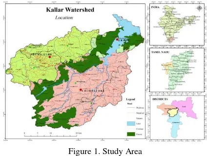
The Kallar watershed situated in Eastern part of Western Ghats stretching from West to the East. It is part of Bhavani river basin, which is the main in Moyar and Bhavani River. It is located between 11˚17’0” to 11˚31’0” N Latitude and 76˚ 39’ 0” to 77˚ 8’ 45” E Longitude and covers an area of 1281.24 Sq.Km. It comprises of three districts, The Nilgiris, Coimbatore and Erode, 6 taluks (Coonoor, Kothagiri, Udhagamandalam, Mettupalayam, Coimbatore north, and Sathyamangalam); and 89 Revenue villages, Figure 1.
Figure 1. Study Area
2.2 Physiographic and Physical setup
The maximum and minimum elevation encountered in the watershed about 177m and 2615m above MSL, Figure 2. About 50% of areas are mountains covered with diverse plant communities that form various types of forest and other agricultural activities, especially Tea, coffee plantation, vegetables and orchards, which are normally cultivated in the upper and the lower area. The climate of this area is temperate and salubrious for more than half of the year. The average day temperature of the sub watershed is 20.15° C to 30° C and the average rainfall is about > 1400 mm. The winter is relatively cool. The maximum rainfall is received during the month of October and November. The Kallar streams flow from Southwest to Northeast and it connects the Bhavani River, which finally joins with Bhavanisagar Dam, it was built in the Northeastern part of the watershed, which is primarily serves as source of irrigation and hydroelectric power generation. The area covered by clay soil, loam soil and rock outcrop on steep to narrow sloping landform. Geomorphologically, the watershed is
characterised by steep structural hills, denudational hills, narrow gorges, and intermountain valleys. Geologically, charnockite and fissile hornblende-biotite gneiss covers major portion of the study areas. The watershed and sub watershed boundary has been demarcated using drainage network and contour crossing.
Figure 2. Physiography
3. DATA AND METHODOLOGY
3.1 Data
The present study has made use of six thematic layers (factors) such as elevation, slope angle, land use, soil texture, precipitation, and NDVI for the preparation of annual average soil loss and erosion risk map. In this study the Survey of India (SOI) toposheets 58 A/11, 15, 16 and 58E/3 & 4, landsat 8 images (Feb 2014, FCC), and precipitation data (1982 - 2012) from Indian Meteorological Department (IMD), Land use from bhuvan portal (2011-12) have been used to create these thematic layers. The working scale of geographic maps was chosen at 1:50,000. ArcGIS 10.1 and Erdas 9.2 were used to prepare thematic maps and layout.
3.2 Methodology
All the collected data were converted into a raster grid with 30 m × 30 m cells for the use. The total cell number is 13, 72,202 for this study. Using rainfall data of Indian Meteorological Department (IMD), rainfall erosivity (R) map of the area was produced by applying interpolation method. Soil texture (K) map was prepared from block level soil report; the contours with 20 m intervals were digitized from extracted SOI toposheet, and generated the Digital Elevation Model (DEM). Using DEM as input the Slope angle (LS) map was generated. Land use / Land cover map was prepared from bhuvan portal. The NDVI was generated from landsat 8 image. Revised Universal Soil Loss Equation (RUSLE) model were adopted for this study and detail of model and processing has explain in modelling part.
4. MODELLING SOIL EROSION AND LOSS
S.K. Saha. Soil erosion prediction and assessment has been a challenge to researchers since the 1930s’ and several models have been developed (Lal, 2001). These models are categorized as empirical, semi-empirical and physical process-based models. Empirical models are primarily based on observation and are usually statistical in nature. Semi-empirical model lies somewhere between physically process-based models and empirical models are based on spatially lumped forms of water and sediment continuity equations. Physical process-based models are intended to represent the essential mechanism controlling erosion.
4.1 Multiple Modelling Approach
To estimate soil erosion and to develop optimal soil erosion management plans, many erosion models based on the empirical models, such as Universal Soil Loss Equation (USLE – USDA Agriculture Handbook 282, first published 1965 and updated version was 1978 in USDA Agriculture Handbook 537) & (Wischmeier and Smithl, 1978), Modified Universal Soil Loss Equation (MUSLE – Williams and Berndt 1976), Chemical Runoff and Erosion from Agricultural Management Systems (CREAMS- Knisel 1980), Agricultural Non-point Source pollution model (AGNPS - Young et al. 1989), Revised Universal Soil Loss Equation (RUSLE - Renardet al.1991), Several physically-based erosion models include Water Erosion Prediction Project (WEPP - Flanegan and Nearing 1995), Soil Erosion Model for Mediterranean Regions (SEMMED), Areal Non-point Source Watershed Environment Response Simulation (ANSWERS), Limburg Soil Erosion Model (LISEM - De Roo et al. 1996), European Soil Erosion Model (EUROSEM - Morgan et al. 1998), Revised Morgan, Morgan and Finney model (RMMF - Morgan 2001), Soil and Water Assessment Tool (SWAT), and Simulator for Water Resources in Rural Basins (SWRRB), etc. were used in regional scale assessment. The various techniques and methods used for the soil erosion spatial vulnerability assessment and quantification of soil loss can be found in (Lal, 1994; Ni and Li, 2003; Lee, 2004; Dabral et al. 2008; Rahman et al. 2009; Zhang et al., 2009; Kim et al., 2012; Vijith et al., 2012; Alexakis et al., 2013; Arar and Chenchouni, 2013; Khosrokhani and Pradhan, 2013; Naqvi et al., 2013; and Rozos et al., 2013). Each model has its own characteristics and application scopes (Boggs et al., 2001; Lu et al., 2004; Dabral et al., 2008; Tian et al., 2009). USLE, RUSLE, RUSLE2 & RUSLE-3D, model has been widely used for spatial prediction of soil loss and erosion risk potential, because of its convenience in application and compatibility with GIS (Millward and Mersey, 1999; Jain et al., 2001; Lu et al., 2004; Jasrotia and Singh, 2006; Dabral et al., 2008; Kouli et al., 2009; Pandey et al., 2009; Bonilla et al., 2010., Parket al.2011, Kumar, S., Kushwaha, S. P. S., 2013 and Balasubramani K et al., 2015).
4.2 Revised Universal Soil Loss Equation
RUSLE is a science based tool that has been improved over the last several years. It is a computation method which may be used for site evaluation and planning purposes and to aid in the decision process of selecting erosion control measures. It provides an estimate of the severity of erosion.
4.2.1 RUSLE Model Description and Limitations: Erosion is a function of erosivity and erodbility. The power of erosion agent to erode is designated as erosivity (raindrop impact, water drops falling from plant canopy, and surface runoff) and the susceptibility (inverse of resistance) of the soil
to erosion is its erodibility. RUSLE factors contain both an erosivity effect and an erodibility effect. Erosivity – RKLSCP, Erodibility – KLC.
The RUSLE model calculates potential average annual soil loss (A) as follows:
A=R*K*LS*C*P (1)
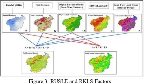
Where A is the computed spatial average annual soil loss, usually on yearly basis (t/ ha-1 /y-1); R is the rainfall-runoff erosivity factor (MJ mm/ha-1/h-1/y-1); K is the soil erodbility factor (t/ ha /h /ha-1 / MJ-1 mm-1); LS is the slope length-steepness factor (dimensionless); C is the cover management factor (dimensionless); and P is the conservation practices factor (dimensionless) Figure 3.
Figure 3. RUSLE and RKLS Factors
In examining the RUSLE variables the equation can be broken down into two parts: 1) environmental variables and 2) management variables (Hickey et al, 2005). The environmental variables include the R, K, L, and S factors. These variables remain relatively constant over time. The management variables include the C and P factors and may change over the course of a year or less. The RUSLE model can predict erosion potential on a cell-by-cell basis, which is effective when attempting to identify the spatial pattern of soil loss present within a large region. GIS can then be used to isolate and query these locations to identify the role of individual variables in contributing to the observed erosion potential value (Shi et al, 2002).
4.3 Model Input Processing and Factor Generation
4.3.1 Rainfall Erosivity (R): The R factor represents the erosivity of the climate at a particular location. An average annual value of R is determined from historical weather records and is the average annual sum of the erosivity of individual storms. R-value is greatly affected by the volume, intensity, duration and pattern of rainfall, whether for single storms or a series of storms, and by the amount and rate of the resulting runoff. Areas with low slope degree have low erosivity R values which imply that flat areas would increase the water ponding on the surface, thus protecting soil particles from being eroded by rain drops. Large numbers of R factor indicate more erosive weather conditions. A period of 20 - 25 year is recommended for computing the average R (Wischmeier and Smithl, 1978), the annual and monthly precipitation data of 12 weather stations for 30 years (1982 - 2012) collected from Indian Meteorological Department (IMD) were used for calculating R-factor using the following relationship equations.
The original equation of (R) uses the kinetic energy of the rain and requires measurements of rainfall intensity (Wischmeier & Smith, 1978) equation (2):
K Ec I30
R= (2)
This direct method of Wischmeier and Smith can only be applied in areas equipped with autographic recorders. An alternative formula developed by Wischmeier and Smith (1978) and modified by Arnoldus (1980) involves only annual and monthly precipitation to determine the R factor equation (3).
12 2 Pi = monthly rainfall (mm) P = annual rainfall (mm)
Present study 30 years of (1980 – 2010) average annual rainfall data has used to calculate and, they were interpolated over the whole watershed using geostatistic model (spline), the average annual R factor values, the range 251.54 to 798.59 MJ mm/ha-1/ h-1/ y-1, Figure 4.
Figure 4. Rainfall Erosivity (R)
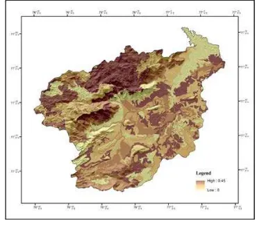
4.3.2 Soil Erodibility (K): Soil erodibilty depends on soil and, or geological characteristics, such as parent material, texture, structure, organic matter content, porosity, catena and many more (Schwab, Fangmeier, Elliot, & Frevert, 1993). Generally, soils become of low erodibility if the silt content is low, regardless of corresponding high content in the sand and clay fractions (Mhangara et al, 2012). In this study Soil texture map were extracted from soil survey data, tamil nadu, was used for K factor. Major soil textural classes found in the areas are clay loam, clay, loamy sand, loamy, sandy clay, sandy clay loam, and sandy loam. The corresponding K values for the soil types were identified from the soil erodability nomograph (USDA1978) by considering the particle size, organic matter content, and permeability class. The estimated K values for the textural groups vary from 0.14 (sandy clay), 0.15 (loamy), 0.20 (clay loam), 0.27(sandy clay loam), 0.28 (clay) and 0.37 (sandy loam) Figure 5.
Figure 5. Soil Erodbility (K)
2
* (0.065 0.045. 0.0065.
22.13 )
CS
LS=PowFA m X + S+ S
(5)
Where FA = flow-accumulation CS = cell size
The flow-accumulation was derived from ASTERGDEM. The LS factor derived is shown in Figure 6, and the value ranges from 0 to 69, with mean and standard deviation of 14.46 and 10.87, respectively.
Figure 6. Slope Length and Steepnes (LS)
4.3.4 Crop Management Factor (C): The Cover Management factor is used to determine the relative effectiveness of soil and crop management systems in terms of preventing or reducing soil loss. The C factor indicates how conservation plans will affect the average annual soil loss and how that soil loss potential will be distributed in time during construction activities, crop rotations or other management schemes (Van der Knijff J M et al. 2000). Soil loss is very sensitive to vegetation cover with slope steepness and length factor (Renard and Ferreira 1993; Benkobi et al., 1994; Biesemans et al., 2000). High C factor values indicate more vulnerability to soil erosion, as they are considered to be unprotected barren land. In the present study, Normalized Difference Vegetation Index (NDVI)-based assessment of C factor was carried out by the equation:
exp
( )
NDVI C
NDVI
α
β
= −
−
(6)
Where αand β are unit less parameters that determine the shape of the curve relating to NDVI and the C factor. Van der Knijff et al. (2000) found that this scaling approach gave better results than assuming a linear relationship, and the values of 2 and 1 were selected for the parameters α and β, respectively. This equation is effectively used by many researchers for finding out the spatial distribution of C factor (Kouli et al. 2009; Prasannakumar et al.2012). In the present analysis, the C factor ranges between 0.6 to 1.32, Figure 7.
Figure 7. Cover Management Factor (C)
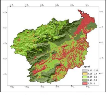
4.3.5 Conservation practice Factor (P): The P-Factor is known as the support practice factor. It reflects the effects of practices that will reduce the amount and rate of the water runoff and thus reduce the amount of erosion. The P factor represents the ratio of soil loss with a specific support practice to the corresponding soil loss with up and down slope (Contour) tillage (Wischmeier and Smith1978; Renard et al. 1997; Dabral et al.2008). Common support practices are: cross slope cultivation, contour farming, strip cropping, terracing, and grassed waterways. In the present study, the P factor map was derived from the land use/ land cover and support factors Figure 8. The values of P factor ranges from 0 to 1, in which the highest value is assigned to areas with no conservation practices (open areas and grasslands), and minimum values given to built-up land and plantation area with contour cropping.
Figure 8. Conservation practice (P)
5. MODELING SOIL EROSION AND LOSS
5.1 Soil Loss
watershed ranges from 0 – 398.58 t/ h-1/y-1 Figure 9. The estimated pixel level soil loss rate was classified into five classes and the spatial distribution of soil loss is given in Figure 10. The classified soil loss map shows that 8.68% of the total area falls under the Nil with tolerable rate of <10 t/h-1/y-1, followed by 41.93% of the total area comes under low soil loss with rate of soil erosion 10- 50 t/h-1/y-1. The critical soil loss occupies 3.82 % of the total area, losing more than 300 ton/h-1/ y-1. Other soil loss categories, like moderate and high covers 33.95% and 11.59 % of the total area with average annual soil loss < 50 and < 300 t/h-1/y-1 respectively table 1.
Figure 9. Annual Average Soil Loss
Figure 10. Soil Erosion Severity Classes
Soil erosion severity
classes
Area in Sq.Km
Annual average soil erosion rate (t/h-1/y-1)
Area in (%)
Nil 45.08 < 10 8.68
Low 610.90 10 - 50 41.93
Moderate 439.97 50 - 150 33.95
High 150.25 150 -300 11.59
Critical 49.67 > 300 3.83
Table 1. Soil erosion severity classes with average annual soil erosion rate
The results were correlated with similar studies carried out in different parts of the Western Ghats and surrounding areas of present sub watershed, (CWRDM, 1997; Matsuura, 2000; M.
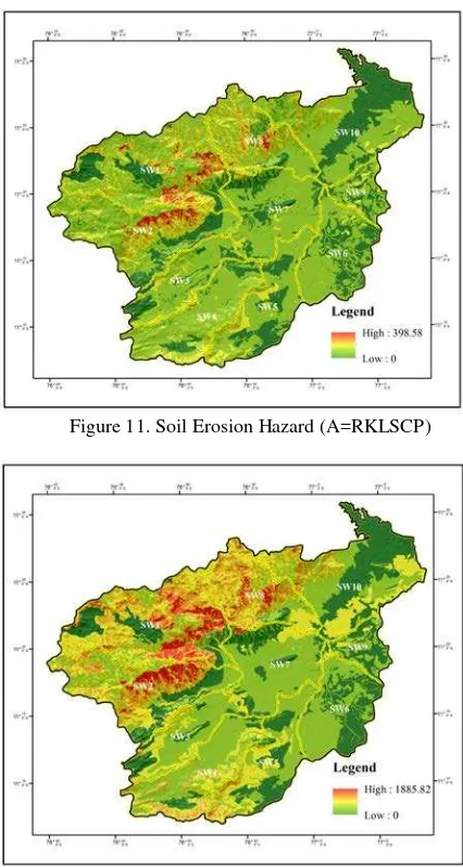
Ramalingam et al, 2002, Prasannakumar et al., 2011). Further computed values of R, K, LS, C and P were classified in to two categories, soil erosion hazard (A=RKLSCP) Figure 11, and Soil erosion susceptibility (A=RKLS) Figure 12, have been computed. To provide some insights into real variations of these values and present sub watershed wise lowest and highest values for soil erosion susceptibility and hazard was computed. However, RKLS values indicate the likely loss of Soil if no crop management and erosion control practices are undertaken. The lowest values of RKLS represent figures for plains (flat to gentle) and the highest for those of the hills. On the other hand, RKLSCP values indicate the loss of soil in the plains (the lowest values) when crop management erosion control practices and the loss of soil in the hills (the highest values) where such practices as those of the conservation practices are also implemented.
Figure 11. Soil Erosion Hazard (A=RKLSCP)
Figure 12. Soil Erosion Susceptibility (A=RKLS)
of land where soil loss is critical. It is understood then that functions of C and P are factors that can be controlled and thus can greatly reduce soil loss through management and conservational measures. Since it is an empirical and traditional model to predict the estimation of average annual soil loss, in future scenario uses of advance technological based approaches like LiDAR and High resolution data’s will be highly effective way to estimate the annual soil loss.
ACKNOWLEDGEMENTS
I would like to acknowledge the Department of Geography, Bharathidasan University and UGC - Basic Science Research Fellowship scheme for aiding me to carry out my research work.
REFERENCES
Angima, S.D., Stott, D.E., O’Neill, M.K., Ong, C.K., Weesies, G.A., 2003. Soil erosion prediction using RUSLE for central Kenyan highland conditions. Agriculture, Ecosystems and Environment 97 (1-3), 295-308.
Alexakis D.D, Hadjimitsis D.G, Agapiou A 2013. Integrated use of remote sensing, GIS and precipitation data for the assessment of soil erosion rate in the catchment area of “Yialias” in Cyprus. Atmos Res Perspect Precipitation Sci I 131:108–124.
Arar A, Chenchouni H 2013. A simple geomatics-based approach for assessing water erosion hazard at montane areas. Arab J Geosci 7(1):1–12
Abdul Rahaman, S., Aruchamy, S., and Jegankumar, R. 2014, Geospatial Approach on Landslide Hazard Zonation Mapping Using Multicriteria Decision Analysis: A Study on Coonoor and Ooty, Part of Kallar Watershed, The Nilgiris, Tamil Nadu, Int. Arch. Photogramm. Remote Sens. Spatial Inf. Sci., XL-8, 1417- 1422.
Balasubramani K, Veena Mohan, Kumaraswamy K, and Saravanabavan V., 2015. Estimation of soil erosion ina semi-arid watershed of Tamil Nadu (India) using revised universal soil loss equation (rusle) model through GIS. Modeling Earth Systems and Environment, vol 1:10.
Dabral, P.P., Baithuri, N., Pandey, A., 2008. Soil erosion assessment in a hilly catchment of North Eastern India using USLE, GIS and remote sensing. Water Resources Management 22, 1783 - 1798.
Desmet, P., Grovers, G., 1996. A GIS procedure for automatically calculating the USLE LS factor on topographically complex landscape units. Journal of Soil and Water Conservation 51(5), 427-433.
Dunn, M., Hickey, R., 1998. The effect of slope algorithms on slope estimates within a GIS. Cartography 27 (1), 9-15.
El-Swaify S. A.,1997, Factors Affecting Soil Erosion Hazards and Conservation Needs for Tropical Steep Lands, Soil Technology, vol. no. 11 (1), page no. 3-16
Jain, S.K., Kumar, S., Varghese, J., 2001. Estimation of soil erosion for a Himalayan watershed using GIS technique. Water Resources Management 15, 41-54.
Jasrotia, A.S., Singh, R., 2006. Modeling runoff and soil erosion in a catchment area, using the GIS, in the Himalayan region, India. Environmental Geology 51, 29-37.
Khosrokhani M, Pradhan B., 2013. Spatio-temporal assessment of soil erosion at Kuala Lumpur metropolitan city using remote sensing data and GIS. Geomatics Nat Haz Risk. doi:10.1080/19475705.2013.794164
Kim S.M, Choi Y, Suh J, Oh S, Park H.D, Yoon S.H., 2012. Estimation of soil erosion and sediment yield from mine tailing dumps using GIS: a case study at the Samgwang mine, Korea. Geosyst Eng 15(1):2–9
Kouli, M., Soupios, P., Vallianatos, F., 2009. Soil erosion prediction using the Revised Universal Soil Loss Equation (RUSLE) in a GIS frame-work, Chania, Northwestern Crete, Greece. Environmental Geology 57, 483-497.
Kumar, S., and Kushwaha, S. P. S., 2013, Modelling Soil Erosion Risk Based on RUSLE-3D using GIS in a Shivalik Sub-watershed, Journal of Earth System Science, Volume 122, Issue 2, pp 389-398.
Lal, R., 2001. Soil degradation by erosion. Land Degradation & Development, 12: 519 –539.
Lee S., 2004. Soil erosion assessment and its verification using the Universal Soil Loss Equation and geographic information system: a case study at Boun, Korea. Environ Geol 45:457–465
Millward, A.A., Mersey, J.E., 1999. Adapting the RUSLE to model soil erosion potential in a mountainous tropical watershed. CATENA 38 (2), 109-129.
Mhangara. P, Kakembo. V and Lim. K., 2012. Soil Erosion Risk Assessment of the Keiskamma Catchment, South Africa Using GIS and Remote Sensing, Environmental Earth Science, Vol. 65, No. 7, 2087-2102.
Moore, I., Burch, G., 1986. Physical basis of the length-slope factor in the Universal Sol Loss Equation. Soil Society of America Journal 50, 194-1298.
Narayan VVD, Babu R., 1983. Estimation of soil erosion in India. J Irrig Drain Eng 109(4):419–434
Naqvi HR, Mallick J, Devi LM, Siddiqui MA., 2013. Multi-temporal annual soil loss risk mapping employing Revised Universal Soil Loss Equation (RUSLE) model in Nun Nadi Watershed, Uttrakhand (India). Arab J Geosci 6(10):4045–4056
Ni JR, Li YK., 2003. Approach to soil erosion assessment in terms of land-use structure changes. J Soil Water Conserv 58(3):158–169
Pandey A, Chowdary V.M, Mal B.C., 2007. Identification of critical erosion prone areas in the small agricultural watershed using USLE, GIS and remote sensing. Water Res Manag 21:729–746
Ramalingam M, Venugopal K, Zaffar Sadiq, Shanmugam M., 2002. Management of Natural Resources through NRIS – A Case Study. Indian Cartographer, MMLP – 05: 310-313
Rozos D, Skilodimou H.D, Loupasakis C, Bathrellos G.D., 2013. Application of the Revised Universal Soil Loss Equation model on landslide prevention. An example from N. Euboea (Evia) Island, Greece. Environ Earth Sci 70(7):3255–3266
Renard K.G and Ferreira V.A.,1993. RUSLE model description and database sensitivity. Journal of Environmental Quality 22(3), 458–466.
Sharma, A., 2010. Integrating terrain and vegetation indices for identifying potential soil erosion risk area. Geo-Spatial Information Science 13 (3), 201-209.
Srinivas, C.V., Maji, A.K., Reddy, G.P.O., Chary, G.R., 2002. Assessment of soil erosion using remote sensing and GIS in Nagpur district, Maharashtra for prioritisation and delineation of conservation units. Journal Indian Society of Remote Sensing 30 (4), 197-212
SinghG, BabuR, Narain P, BhusanLS, Abrol IP., 1992. Soil erosion rates in India. J Soil Water Conserv 47(1):97–99
Van der Knijff J M, Jones R J A, Montanarella L., 2000. Soil Erosion risk Assessment in Europe, European Commission, European Soil Bureau.
Van Remortel, R.D., Maichle, R.W., Hickey, R.J., 2004. Computing the LS factor for the Revised Universal Soil Loss Equation through array-based slope processing of digital elevation data using a C++ executable. Computers and Geosciences 30, 1043-1053.
Vijith H, Suma M, Rekha VB, Shiju C, Rejith PG., 2012. An assessment of soil erosion probability and erosion rate in a tropical mountainous watershed using remote sensing and GIS. Arab J Geosci 5(4):797– 805
Zuazo, Victor H.D. & Pleguezuelo, Carmen R.R., 2009, Soil-Erosion and Runoff Prevention by Plant Covers: A Review In Lichtfouse, Eric et al. Sustainable Agriculture. Springer, page. no. 785.
Anon (2008) Annual report (2007–08): Ministry of Agriculture, Govt. of India.
Anon (2009) State of environment report. Ministry of Environment and Forest, Govt. of India.
Saha S.K. Kudarat M Bhan, S.K., 1992 .Erosion soil loss prediction using digital satellite data and Universal soil loss equation –soil loss mapping in siwalik hills in India .In book on. “Application of Remote Sensing in Asia and Oceanic- Environmental change monitoring ” (Ed.Shunji mural) ; Phb. Asian Association on Remote sensing , 369-372.