ANALYSIS
The mineral economy: how prices and costs can falsely
signal decreasing scarcity
Douglas B. Reynolds *
Department of Economics,Uni6ersity of Alaska Fairbanks,PO Box756080,Fairbanks,AK99775-6080,USA
Received 16 February 1999; received in revised form 16 July 1999; accepted 20 July 1999
Abstract
Natural resource prices and costs of extraction have declined simultaneously with increasing quantities of extraction for a long time. In a Hotelling sense this indicates decreasing scarcity since low cost resources normally would be used first and quantities of extraction normally would decrease over time. The main reason for the trend being opposite to Hotelling characteristics is usually thought to be due to technological innovation. However, an alternative reason for decreasing costs and prices and increasing quantities of extraction may be due to Georgescu-Roegen’s [Georgescu-Roegen, Nicholas, 1972. Energy and economic myth. In: Georgescu-[Georgescu-Roegen, Nicholas (Ed.), Energy and Economic Myths: Institutional and Analytical Economic Essays. Published 1976, Pergamon Press, New York, pp. 3 – 36] concept of ‘Bonanza’ where there is only the appearance of decreasing scarcity. Norgaard’s [Norgaard, R.B., 1990. Economic indicators of resource scarcity: a critical essay. J. Environ. Econ. Manage. 19(1), 19 – 25] ‘Mayflower’ problem can be used to model an alternative neo-classical approach to resource extraction and scarcity. In this paper, a model of resource exploration is developed where the explorer does not know total reserves of the resource base as he searches for and extracts the natural resource. The explorer never entirely knows how big the resource base is but does gain information about the potential location of new reserves as discovery proceeds. That reduces exploration costs. The lower exploration costs can cause the price to fall over time, until eventually scarcity of the resource causes the price to rise. The true scarcity is only revealed towards the end of exhaustion. The model shows that it is possible to have several years of increasing production simultaneous with lower prices and costs until a sudden, intense price rise occurs with a huge cut in production. When technology is able to cut costs and increase the reserve base, the decline in prices and costs and the increase in production can last longer. However, even with better technology, it is still possible for a sharp increase in price as long as demand is growing faster than technological innovation. The problem is that the true size of the resource base is never known. Society does not know if technology is actually overcoming scarcity or not until demand for a resource outstrips supplies. It is even possible for a price shock of incredible magnitude to surprise an economy within one or two years after a hundred years of declining prices and increasing production. © 1999 Elsevier Science B.V. All rights reserved.
www.elsevier.com/locate/ecolecon
* Tel.: +1-907-474-6531; fax:+1-907-474-5219. E-mail address:[email protected] (D.B. Reynolds)
Keywords:Resources; Scarcity; Technology; Exploration; Information; Hubbert; Norgaard’s Mayflower problem
1. Introduction
According to Hotelling (1931) there are three things we can say about resource extraction for a finite resource. (1) Firms will always try to extract low cost resources before high cost resources, causing resource extraction costs to increase over time. (2) In general, greater scarcity of in-situ reserves increases the value of a resource causing the price to increase over time. (3) Since the price of a resource increases over time, then demand and production should decrease over time. Bar-nett and Morse (1963), and more lately Scott and Pearse (1992) and Simon (1996), show that none of these theoretical trends have occurred. Costs of extraction and prices of natural resources have mostly decreased over time, not just in recent years, but in many cases for decades. Quantities extracted and produced of most natural resources have also increased over the same long time frame. The only logical explanation is that tech-nology and substitutes are in fact more powerful than scarcity.
In this paper is shown an alternative model for scarcity based on the Mayflower problem of Nor-gaard (1990) which demonstrates how it is possi-ble for there to appear to be long trends of decreasing scarcity only to have a sudden and dramatic increase in scarcity. The model here shows that long-run resource exploration cost and resource price declines simultaneous with increas-ing resource extraction, do not necessarily signify decreasing scarcity. The paper shows that the true power of technology in overcoming scarcity may be difficult to determine. It is also shown how price and cost measures of scarcity may fail even when prices and costs have declined for many years.
Hall and Hall (1984) define scarcity in terms of the cost of extracting a resource, which is based on Hotelling’s original concepts. Malthusian scarcity is where in-situ stocks are finite, and Ricardian scarcity is where stocks are not finite, but costs of extracting them increase as you
ex-tract more. Concentrating on Malthusian scarcity, Hall and Hall define Malthusian Stock Scarcity (MSS) where resource stocks are finite but are of uniform quality so that the cost of producing them stays relatively constant with constant tech-nology. However, instead of looking at the cost of extraction to determine scarcity, this paper will look purely at the costs of exploration. Extraction costs will be zero. The assumption of zero extrac-tion costs can be modified later, nevertheless, this assumption changes the emphasis of determining scarcity away from the costs of producing a re-source and toward the cost of finding a rere-source. Norgaard looks at the difficulty of exploring for resources in the ‘Mayflower’ problem where information about the location of low cost natu-ral resources is incomplete. When the Mayflower pilgrims came to America, they settled at the first most convenient location possible in New Eng-land even though the soil there was not as good as the soil in, say, the Midwest. If the Mayflower pilgrims had used the available resources opti-mally in a Hotelling sense, they would have taken the Mayflower to the Gulf of Mexico and up the Mississippi River all the way to Iowa in order to start their farms there. Or at least within a gener-ation or two, the new settlers would have moved all their settlements to the Midwest. At least part of the reason that the Mayflower pilgrims and subsequent generations did not go to the Midwest quickly was because they did not know that there was good soil there. Their actions imply that finding information about resource location is an unavoidable cost of the supply of natural resources.
2. Monte Carlo modeling
wells throughout the US starting in 1859, then the super giant East Texas oil field would have been discovered at the very least by 1902, given the historical rate of exploration. East Texas was actually discovered in 1930. Other giant and super giant fields also undoubtedly would have been found earlier by merely drilling exploration oil wells randomly. The problem with the analysis is that Menard and Sharman know something that the early oil explorers did not know, namely, that the East Texas oil field exists. In other words, the Monte Carlo modelers have perfect information that 22 giant oil fields in the US exist before they run their model, but the early oil explorers did not have this information and did not know if even one giant oil field existed until the first one was found. Therefore, consider an alternative set up.
A Monte Carlo model is rather like playing roulette where there are black and red slots on the roulette wheel for the ball to fall into. Black is oil, red is dry. The probability of getting black on a bet that costs the amount of money for drilling an oil well depends on how many black slots there are as a proportion of all the slots. If you were to play the gamble, the expected results are exactly equal to the probability of getting black. How-ever, different roulette wheels, like different coun-tries and different regions, have different probabilities of success. For example, compare finding oil in the Persian Gulf to that of Switzer-land. In other words, there are different roulette tables with different probabilities.
Assume then that there is a large room full of roulette tables, and that gamblers will come into the room to play the tables. Based on their ex-pected probability of winning, they will be more willing to bet on the tables with the higher proba-bility of black since those tables will have a higher expected gain. Now assume one more thing. All the roulette tables are covered and mixed before the gamblers enter the room. In that case, the gamblers do not know which tables have a high proportion of black slots and which have a high proportion of red slots. They do not even know if any tables have any black slots. The gamblers have no idea what their chances of winning are or even if there is anything worth betting on or not.
As the gamblers come into the room with the covered roulette tables, they must try to get infor-mation about what the tables are like. What strategy will they use? Undoubtedly, the gamblers will wait to see what other gamblers do. If one gambler does make a bet and does get a black slot, chances are good that at least that particular roulette table has more black slots. The gamblers race to that table and start betting. However, as the bets are made, every time a slot is hit, it is removed and not replaced. Eventually the black slots are used up and the gamblers will have to leave old tables and start taking their chances on newer tables.
The gamblers do not randomly play on all the roulette tables, as implied by a pure Monte Carlo model. For all they know, all the tables could have only red. There is no way of knowing a priori what the probability is that any black slots exist. In this situation, the gamblers have in their mind a subjective probability of winning at any given table. However, their subjective probability is different than the actual probability of the table. When the gambler goes to a table where previous gamblers won black, he has information to judge the probability that he also will win based on past experience. That is his own subjec-tive probability. It is based on available informa-tion. A gamblers subjective probability will be higher at a table with a past history of winning bets than with an unknown table where there is no history. The subjective probability of getting black at a new table may be lower or even much lower than the actual probability of getting black at that table. Therefore, there is a difference be-tween a gambler’s or a mineral explorer’s subjec-tive probability of finding a mineral and the actual probability of finding a mineral, should he drill a well.
different perspective on how a resource dependent economy will act over time, and on the interpreta-tion of the effect of better technology on scarcity.
3. The mineral economy model
Two economic models describe a resource-based economy in its purest form: the ‘corn’ econ-omy and the ‘hardtack’ econecon-omy explained below. For a complete analysis of these models, see Page (1979). We can call a third type of resource model the ‘mineral’ economy. The mineral economy model is similar to a hardtack economy model except that the mineral — the hardtack — is hidden. The hidden hardtack must be explored for and extracted before it can be used. To explain the models, consider Robinson Crusoe stranded on a deserted island. In the corn economy sce-nario, he has some corn with him. He can choose to use varying amounts of the corn to either plant or eat depending on what his intertemporal pref-erence is. If he eats more corn now, he has less corn to plant for future output. On the other hand, if he plants more corn, he will have more future output but less to eat right now. In an infinite horizon world, such as a tribe of constant population on the island, a corn economy can last indefinitely.
In the second scenario, Crusoe is faced with a much more sobering possibility of only having a finite amount of hardtack. Again, depending on his personal preference, his years of life and the amount of hardtack he has, he faces several sce-narios for exhausting that hardtack. He can choose to eat more now or save his stock and eat more later, but his reserves are limited. He may even not survive long if his supply is too small. If we extend Crusoe’s life indefinitely by replacing him with a tribe on the island with a constant population and still a finite amount of hardtack, then that society faces the inevitable dilemma of sooner or later running out of hardtack and dying off. Better technology, though, could overcome such a grave scenario.
However, neither of these scenarios for Robinson Crusoe parallels the real world where our economies are to a large degree based on
underground non-renewable non-recyclable re-sources, such as oil, coal and natural gas. In the real world, unlike a hardtack economy, these nat-ural resources are not stored in such a manner so that we can quantify them costlessly, the way we can quantify hardtack stores costlessly. Rather, many natural resources are hidden from the econ-omy until they are found. The hidden resources create an unavoidable cost for finding the miner-als. That is an exploration cost. Even if extracting the mineral is costless, there is still an exploration cost implied by the search process that influences the rate of extraction. Using the characteristics of the Mayflower problem, we can create a model for the cost of exploration over time and then use that model to analyze scarcity and how powerful technology really is for overcoming scarcity.
Consider a situation where Robinson Crusoe lands on a deserted island with no food. Assume that previous shipwrecks with no survivors have left hardtack on the island. If Crusoe is able to find these old shipwrecks and the hardtack on them, he can survive by eating the lost hardtack. However, let us further assume that these previ-ous shipwrecks happened many years before Cru-soe’s shipwreck, such that all the ships have been buried deep in the sand and are not visible from the surface. Crusoe can survive by eating this leftover hardtack, which is his ‘mineral’ resource, if Crusoe can find it. This situation is the mineral economy. In the mineral economy assume there is MSS where the resources are of constant quality and even free to extract. The only problem is knowing how much resources there are and find-ing them.
the covered roulette wheels all going to the one table where there was a black slot found and betting on it. Therefore, with this new informa-tion about one ship’s locainforma-tion, Crusoe will be better able to find other ships and his cost of searching will decrease. The more hardtack that Crusoe finds, the more information he has, and the easier it is to find even more hardtack.
Eventually though, because the supply of hard-tack is finite, depletion sets in and Crusoe finds less and less hardtack. Therefore, even though Crusoe has more and more information about where the hardtack is, the depletion of the re-source base creates higher costs of exploration; since it is hard to find the last few remaining stocks the rate of discovery decreases. Crusoe’s supply of hardtack left to be found dwindles until he can no longer survive.
Two long-run forces, then, drive Crusoe’s min-eral economy. First, there is the information effect where the more information Crusoe has about the location of the hardtack, the cheaper it is to find and the more he is able to find. Second, there is the depletion effect where the less hardtack that remains to be found, the costlier it is to find and the less he can find. These forces create a pattern of first an increasing and then a decreasing rate of discovery. Uhler (1976) calls the two opposite forces of information and depletion the informa-tion and depleinforma-tion effects.
4. An exploration information cost model
Assume that Crusoe’s technology for finding and using the hardtack stays constant and actual extraction is costless. Changes to these assump-tions are possible after the basic model is devel-oped. Assume every time Crusoe explores a location for hardtack, he must eathcof hardtack in order to give himself the physical energy to look. This is his cost of exploration effort. If Crusoe searches in 20 locations, he must eat 20 times hc hardtack. Furthermore, assume for sim-plicity that when hardtack is discovered in any one location it is always the same amount of hardtack, call ithd. While most minerals occur in large and small loads or pools rather than
con-stant loads, it is assumed that a large load is the same as a lot of small ones that are near each other. Therefore, hardtack that is left in the ground from previous shipwrecks is always packed in small tins or boxes that are the samehd size. The tins are separate and must be discovered separately. Smith and Paddock (1984) suggest, based on empirical evidence, that minerals such as oil occur in large and small pools or loads and that the largest pools or loads of minerals are usually found first and then subsequently smaller pools and loads are found within one region. However, their empirical evidence is not general enough, since in many cases the largest loads of minerals are not the very first reserves found. For example, the East Texas oil field, Prudhoe Bay, and the great Ghwar oil field in Saudi Arabia were not the first oil fields found even though these are some of the largest fields on Earth. In general, small loads of minerals are found first, then large ones and then small ones again. For Crusoe, it is assumed that each tin is separate and equal, however, large loads of minerals can be simulated by having lots of tins being close to-gether. When one is found others nearby are easy to find. Hence:
hc=pounds of hardtack consumed per
exploration location that is searched, i.e. effort cost.
hd=pounds of hardtack found per exploration location when the exploration is successful.
hdis the pounds of hardtack found in each tin. All tins are assumed constant for all successful exploration locations.
hd\hc
of exploration, and information, which is depen-dent on cumulative discovery.Prmodels Crusoe’s subjective probability of finding more hardtack rather like a probability coin. Every time Crusoe expends effort to search for hardtack at a specific location, his success of finding more hardtack is like flipping a coin. However, the probability of success is not necessarily 50/50. Instead, the prob-ability weight of the coin can be anywhere from 0/100 to 100/0 for success, depending on Crusoe’s subjective probability. That subjective probability depends on information such as how successful previous explorations have been and exploration progress. The subjective marginal benefit of explo-ration for Crusoe is then hd·Pr or, alternatively, the marginal cost is hc/Pr.
In the Monte Carlo game with the gamblers, there was the actual probability of taking a gam-ble on the roulette wheel, which the gamgam-blers did not know, and their own subjective probability of gambling at that table. Like the gamblers in an unknown Monte Carlo simulation, Crusoe too has no idea if there is any hard tack at all under ground or, if there is some, where it is. Neverthe-less, Crusoe will use whatever information he can garner from past experience to choose the best location possible. His subjective probability, Pr, will change as information changes.
There are two distinct aspects of how informa-tion affects Crusoe’s explorainforma-tion process. When Crusoe begins his search for hardtack at the be-ginning of the day, he will have in his mind all possible information about where hardtack may or may not be. He will begin his search at the location where his subjective probability of suc-cess is the highest. That is, Crusoe will explore for hardtack first in the most probable locations. He will continue searching at second and third best locations. Therefore, as the day passes, Crusoe will have a lower and lower probability of success. During the day, however, Crusoe may also gain new information which could help his search. For example, Crusoe may discover hardtack and start to see a pattern about where hardtack usually occurs underground. This may increase his proba-bility of success. Therefore, there are two distinct forces that affect the probability of success. One force is where the old information becomes less
and less useful in helping Crusoe make successful new discoveries. The other force is where new information discovered during the course of ex-ploration helps Crusoe raise his probability of success. In order to understand these two forces better let us separate them and model them differ-ently. For simplicity, assume that Crusoe can only use one set of information during a given day and that any new information he finds he cannot assimilate until the next day. This will separate the effects of information into a short-run (within a day) and a long-run (longer than one day) time frame. In other words, Crusoe will use informa-tion rather like capital. ‘Informainforma-tion capital’ is Crusoe’s accumulated information, i.e. his stock of information. Information capital is like a stock of capital machinery, it cannot change in the short run. Only in the long run can new information be added to the current stock of information, causing the information capital to increase.
4.1. Short-run characteristics of probability
capital declines as effort and therefore output increases. This is similar to how the marginal productivity of capital itself declines as output increases. The effect of the degrading value of old information is to cause a decreasing probability of success. A convenient formula for Pr to model this short-run value of the information capital is the following:
Pr=exp[−Q/L]
Q=Q(S)
where
dQ/dS\0
and Q=the daily quantity discovered or current rate of discovery; S=effort in terms of numbers of searches per day; L=a long run trend parameter.
The short-run probability will act as a decline curve as the rate of discovery increases. The rate of effort,S, is an independent variable chosen by Crusoe, which will determine the rate of discov-ery. If effort increases, discovery increases and probability falls. At the beginning of the day it may take two exploration tries to find hardtack, but as the day wears on, it may take Crusoe ten tries. Therefore, the probability of finding that last tin of hardtack decreases from 50 to 10%, and hence the marginal cost rises. The lower probabil-ity of success is due to the diminishing returns on the current information capital which increases marginal cost. Crusoe will tend to look for hard-tack during the day until his cost of exploration is close to or equal to his benefit of successful discovery,hd. Setting the probability as a function of the rate of discovery rather than effort makes the model easier to work with. The more one discovers the resource during the day, the more one uses the current information capital. The more the current information capital is used, the less valuable it is. The less valuable the informa-tion capital is, the lower the probability of suc-cess. Therefore marginal cost rises.
4.2. Long-run characteristics of probability
Recall in the Monte Carlo situation above that initial gambles, like initial efforts to find a
re-source, are very unsuccessful due to a lack of knowledge, and therefore a great deal of effort is used to find only a small amount of resource. Eventually, however, with greater information, it takes fewer efforts to find a given amount of resource. Therefore, in the long-run, new informa-tion will increase the informainforma-tion capital and in-crease the probability of success, such that the probability of finding the mineral will increase. Concurrently, however, there is depletion. In ad-dition to long-run information gains, the deple-tion effect will cause less of a resource to be found. As a resource depletes to nothing, the probability of finding more of that resource must also decline. Therefore, in the long-run, two ef-fects on probability are modeled: the information effect and the depletion effect. See Uhler (1976).
With greater information capital Crusoe can find more hardtack for a given level of effort. Greater cumulative discovery implies greater in-formation capital, which will cause a higher prob-ability of success. This is the information effect. However, with greater depletion, Crusoe will find less hardtack with a given level of effort. Greater cumulative discovery equates to less remaining resources in the ground available to find, which will cause a lower probability of success. This is the depletion effect. The information effect will dominate initially, and the depletion effect will dominate subsequently. The probability weight functions as a whole shifts first outward and upward and then inward and downward with cumulative discovery. The result is a small – large – small sequence of the discovery and extraction of hardtack in the long-run. These long-run effects on probability are modeled using cumulative discovery.
indicator of information capital as cumulative exploration efforts. The benefit of using cumula-tive discovery rather than cumulacumula-tive effort is that one variable can be used for both the in-formation and depletion effects more simply.
Greater information capital shifts the proba-bility weight function higher. That shift is an information effect shift, where greater cumula-tive discovery implicitly signals greater informa-tion capital. As the stock of undiscovered reserves depletes to zero, though, the probability of finding new hardtack must eventually become zero because there is no more hardtack left to find. The depletion effect then is where less hardtack reserves make it more difficult to find new hardtack causing the probability weight function to shift down. The depletion effect de-pends explicitly on greater cumulative discovery because higher cumulative discovery equates to a lower stock of remaining undiscovered re-serves.
In order to model the information and deple-tion effect, assume the long-run trend parame-ter, L, shifts the probability function Pr in the manner explained above. A likely equation for the trend is Hubbert’s life cycle hypothesis (Hubbert, 1962). Hubbert’s life cycle hypothesis, which was used to explain the long-run trend of oil production in the US, ideally models a min-eral economy faced with the Mayflower prob-lem. Hubbert’s model has a small – large – small sequence of discovery and production of a min-eral that would be expected in the minmin-eral econ-omy. For an economic analysis of Hubbert, see Cleveland (1991), Cleveland and Kaufmann (1991), McCabe (1998), and Edwards (1997). Hubbert’s original model using L as the trend for current discovery is a time dependent logis-tics curve as follows:
L=aU{1+exp[−a(t−t0)]} −2
exp[−a(t−t0)] (1)
where a=an amplitude parameter. This deter-mines the height and width of the Hubbert curve; t0=the time at which the peak in pro-duction occurs; t=time; U=ultimately recover-able reserves; L=the trend of the rate of discovery.
However, it is possible to subsume the time element of Hubbert’s logistics curve in order to make it a pure cumulative discovery model that can be used to measure the combined effects of information and depletion. Hubbert’s cumulative discovery model is as follows,
CQD=U/{1+exp[−a(t−t0)]}
which can be rewritten as
(t−t0)={ln[U/CQD−1]}/ −a (2)
where CQD=cumulative discovery. Substituting Eq. (2) into Eq. (1) gives
L=a·CQD−a·CQD2/U (3)
which can be called the Hubbert trend.
Wiorkowski (1981) developed a range of lo-gistics curves similar to Hubbert’s life cycle curve, using what is called the Richards function (Richards, 1959). From Wiorkowski and Hub-bert, a generalized trend in terms of cumulative discovery can be used to describe L over time. The generalized Hubbert trend is as follows.
L=a×CQD×U(m−1)/
m−a×CQDm×CQD/U
×m
and, when m=0,
L=a×CQD×lnU/U−a×ln CQD×CQD/U
where m=shape parameter, −1BmB .
Eq. (3) was Hubbert’s original trend where
m=1.
5. A mineral market simulation
Since Crusoe does not know how much hard-tack is under the ground — it could be one mil-lion times his most opulent lifetime consumption or only a weeks worth of food — he cannot per-form an intertemporal maximization. If Crusoe’s discount rate is zero, he simply lives at a subsis-tence level. However, for any other discount rate above zero, he just does not have enough infor-mation to maximize utility. Nor can a tribe of constant population. As long as a tribe has a rate of discount greater than zero, they cannot use the Hotelling principle since they do not know if the resource base will last a thousand generations or less than one. Therefore, a simple Crusoe model cannot be solved. However, if we assume that Crusoe or a tribe believes that the resource is so vast that it verges on being infinite, i.e. that the probability of discovery always goes up in the long run, then there would be no Hotelling rent. The resource is seemingly renewable. Crusoe will each day explore up to the point where marginal cost equals hd. Consider this possibility more generally.
Assume instead of Crusoe by himself that there is a large economy and that there is a mineral industry for one particular essential natural re-source input into that economy. The market for the mineral is within a larger market place. The marginal cost of finding the mineral for all firms in the industry is:
MC=Ec/hd×Pr
where Ec=cost of effort in the industry; MC= aggregated marginal costs of the industry.
Pr=exp(−Q/L)
Pr is determined by the industry-wide rate of discovery. When the industry extraction rate, Q, increases, Pr decreases due to industry-wide di-minishing returns to information capital. Note, the industry is made up of many firms and all firms use each others’ information; therefore, this is an efficient market where all information is available to the other players, similar to the Monte Carlo gambling simulation above. Costs are minimized, profits maximized. hd is the
mar-ginal unit of extraction; therefore let hd=1 for convenience. The cost of actual extraction is as-sumed zero. That assumption can be changed to add an extraction cost that also decreases with time, but the general conclusion will be the same. Therefore in this simulation it is assumed that the aggregated marginal cost includes both extraction and exploration costs. In that case:
MC=Ecexp(Q/L) (4)
This gives the following characteristics:
dMC/dCQDB0
when the information effect dominates
and
dMC/dCQD\0
when the depletion effect dominates
In addition technological effects for supply can be added to Eqs. (3) and (4). Let:
Ec=Ecoexp(−Tct)
where Ec0=initial cost of effort in the industry;
Tc=cost technology factor (the percent reduction in costs per year).
Also
U=U0exp(Tut)
where Uo=initial ultimately recoverable reserves;
Tu=ultimately recoverable reserve technology factor (the percent increase in ultimately recover-able reserves per year due to technology).
Consider a simple demand curve for the re-source that reflects a growing economy.
Q=G(P)−1/3 (5)
and
G=G0exp(gt)
where G=economic production of the entire economy;G0=initial economic production of the economy; g=economic growth factor for the economy; P=price for a given quantity demanded.
for a very long time, and they look to continue to fall for a long time, then producers will set P= MC. There will be no Hotelling rent. Producers believe the resource is infinite due to new technol-ogy. When technology is thought to be the cause of a long price decline, then it is easy to conclude that technology will continue to improve indefin-itely and cause prices to fall indefinindefin-itely. In that case, a resource producer maximizes present value, not by withholding exploration for, or ex-traction of, resources, but by producing more now before prices go even lower. The producer maxi-mizes present value simply by producing as much as profitable in the current year irrespective of rent. Producers would generally set P=MC.
Consider a model simulation using the follow-ing values for Eqs. (3) – (5):
U0=100 000 a=0.15 Tu=1% per year, i.e. slower than economic growth G0=500 g=3% per year, i.e. faster than the rate of technological growth of the resourceEc0=1 Ec13=1,Ecis held constant in the initial 13 periods to give the system stabilityTc=5% per year after the first 13 years.
In the simulation, the technology to increase ultimately recoverable reserves is improving at a slower pace than economic growth. However, the effect of technology on the resource base to in-crease its recoverable reserves is unknown to the market and remains unknown until late in the exploration process. Therefore, the market sets
P=MC. In each period,QandPare solved using Eqs. (3) – (5), then the effects of technology are added. Since Eqs. (4) and (5) are indeterminate forQ,Qt−1is used to solve forQt. The difference betweenQt andQt−1is small enough so that the substitution creates no problem.
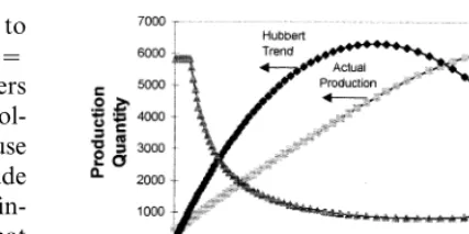
The results of the simulation can be seen in Figs. 1 and 2. In Fig. 1, the supply Hubbert trend (L), the quantity produced (Q) (which is the equilibrium of supply and demand), and price (P) are shown as a function of cumulative production (CQD). Actual production is less than the supply trend potential, i.e. the Hubbert trend, for most of the cycle. It is only after the supply Hubbert trend reaches its point of decrease that production finally gets close to and goes above the Hubbert
Fig. 1. Price, production, and Hubbert supply trend as a function of cumulative production.
trend. The Hubbert supply trend is only the trend
of supply; it does not determine absolute supply. The actual supply can be above or below the Hubbert trend although supply becomes increas-ingly inelastic above the Hubbert trend. Scarcity is revealed only when production goes well above the Hubbert trend. At that point, the price finally starts increasing and production finally starts de-creasing. Before that point, it is not possible to know how forceful technology is for increasing potential reserves. Suddenly, scarcity is revealed but unlike the Hotelling model, there is no forewarning.
In Fig. 2 the price trend is shown as a function of time. Notice that the price, as well as the costs that determine price, which is not shown, decline for many years before the price finally increases. Furthermore, during those price decreases, quan-tities of the resource extracted are constantly in-creasing. In fact, it is possible to model a situation where price decreases and supply quantity in
creases continue for hundreds or even thousands of years before the price finally rises and quanti-ties finally decline. However, the change from one trend to the other can happen within a few years even though the trends before the change over lasted for hundreds of years. In other words, the information effect can dominate the depletion ef-fect for a very long time before depletion finally and dramatically dominates. If you add to the information effect technology, then it takes even longer before depletion dominates. Nevertheless, the power of technology to overcome scarcity is not known until it is revealed late in the cycle.
The problem with using price, cost or quantities produced as a measure of scarcity is that up until the point where demand crosses the Hubbert trend, it is unclear how powerful technology is for decreasing scarcity. Only when prices start actu-ally rising due to the depletion effect can society know how big the Hubbert cycle is and how much technology has stretched the resource base. Before that point in time, the information effect obscures the size of the resource base and the true power of technology for reducing scarcity. An additional problem is that since price declines for a long period of time before the price shock, it is unclear what substitutes for the resource are available and at what price. There has been no gradual increas-ing price and therefore no signal to inventors of when a backstop will need, and no signal to consumers of when the backstop will be needed to be used. The market is not properly prepared for the change over.
However, once the price reaches its lowest level in Fig. 2, producers of the resource will realize that the resource is a lot more scarce than they had previously thought. They will suddenly un-derstand that the price will start increasing and they will cut production in order to maximize intertemporal profit via the Hotelling principle. This cut in production will cause the price shock to be much more severe. In addition, Reynolds (1998) shows that the backstop price of a resource can unexpectedly rise due to the loss of entropy subsidies. It is conceivable that after one-hundred years of price decline and production increase, a resource can have a 10- or 100-fold price increase within a year or two, with a corresponding decline
in production. Given that short-run elasticities of demand and substitution are much more inelastic than long run elasticities, this can create quite a problem for an economy, to say the least.
6. Conclusion
In the Hotelling model, there is perfect infor-mation about the backstop price, the quantity of the resource, the demand for the resource, and the cost of extracting the resource. With perfect knowledge, rent of a resource increases at the interest rate up to the backstop price. Uncertainty theory can be added to the Hotelling model to try to find out how trends of prices and quantities change under various assumptions when the re-source base is unknown. However, if there is enough uncertainty it is almost impossible to use the Hotelling principle. In this model it is shown how the uncertainty of the resource base can obscure the actual trend of scarcity and the true power of technology and create a price shock. Such a price shock can occur after a very long price and cost decrease simultaneous to a long production increase. This model shows theoreti-cally that empirical data on cost and price de-clines as well as data on increases in quantities of extraction do not necessarily imply decreasing scarcity. Indeed, such data may not even be useful for warning about impending price shocks. What is even more foreboding is that once producers do know that scarcity is much greater than previ-ously thought, the price shock will become all the more severe. Resource producers will cut back production due to increasing prices causing prices to increase even further. The so-called backstop price may be much higher than expected espe-cially since the loss of entropy subsidies can make the backstop price increase substantially.
Acknowledgements
References
Barnett, Harold J., Chandler, Morse, 1963. Scarcity and Growth; The Economics of Natural Resource Availabil-ity. Johns Hopkins University Press for Resources for the Future, Baltimore.
Cleveland, Cutler J., 1991. Physical and economic aspects of resource quality, the cost of oil supply in the lower 48 United States, 1936 – 1988. Resour. Energy 13, 163 – 188. Cleveland, Cutler J., Kaufmann, Robert K., 1991.
Forecast-ing ultimate oil resources and its rate of production: in-corporating economic forces in the models of M. King Hubbert. Energy J. 12 (2), 17 – 46.
Edwards, John D., 1997. Crude oil and alternative energy production forecasts for the twenty-first century: the end of the hydrocarbon era. Am. Assoc. Petroleum Geologists Bull. 81 (8), 1292 – 1305.
Hall, Darwin C., Hall, Jane V., 1984. Concepts and measures of natural resource scarcity with a summary of recent trends. J. Environ. Econ. Manage. 11, 363 – 379.
Hotelling, Harold, 1931. The economics of exhaustible re-sources. J. Polit. Econ. 39 (2), 137 – 175.
Hubbert, M.K., 1962. Energy Resources, A Report to the Committee on Natural Resources: National Academy of Sciences, National Research Council, Publication 1000-D. Washington, DC, pp. 54, 61, 67.
Menard, H.W., Sharman, George, 1975. Scientific uses of random drilling models. Science 190 (42), 337 – 343.
McCabe, Peter, 1998. Energy resources — cornucopia or empty barrel? Am. Assoc. Petroleum Geologists Bull. 82 (11), 2110 – 2134.
Norgaard, R.B., 1990. Economic indicators of resource scarcity: a critical essay. J Environ. Econ. Manage. 19 (1), 19 – 25.
Page, Talbot, 1979. Conservation and Economic Efficiency. The Johns Hopkins University Press, for Resources for the Future, Baltimore.
Reynolds, Douglas B., 1998. Entropy subsidies. Energy Pol-icy 26 (2), 113 – 118.
Richards, F.J., 1959. A flexible growth curve for empirical use, J. Exp. Botany 10, 290 – 300.
Scott, Anthony, Pearse, Peter, 1992. Natural Resources in a high-tech economy: scarcity versus resourcefulness. Re-sour Policy 18 (3), 154 – 166.
Simon, Julian L., 1996. The Ultimate Resource 2. Princeton University Press, Princeton.
Smith, James L., Paddock, James L., 1984. Regional model-ing of oil discovery and production. Energy Econ. 6 (1), 5 – 13.
Uhler, R.S., 1976. Costs and supply in petroleum explo-ration: the case of Alberta. Can. J. Econ. 9 (1), 72 – 90. Watkins, C.J., 1992. The Hotelling principle: auto bahn or
cul de sac? Energy J. 13 (1), 1 – 24.
Wiorkowski, J.J., 1981. Estimating volumes of remaining fos-sil fuel resources: a critical review. J. Am. Stat. Assoc. 76 (375), 534 – 547.