www.elsevier.com / locate / econbase
A note on the proper econometric specification of the gravity
equation
*
Peter Egger
Austrian Institute of Economic Research, P.O. Box 91, A-1103 Vienna, Austria
Received 8 February 1999; accepted 13 July 1999
Abstract
This paper sheds some light on the problems associated with random effects gravity approaches. Arguments for the superiority of a fixed effects model are given both along intuitive and econometric lines based on a Hausman test. 2000 Elsevier Science S.A. All rights reserved.
Keywords: Gravity equation; Panel econometrics
JEL classification: C33; F14; F15
1. Introduction
Among the huge empirical literature on gravity models published in the last decade most studies have been done with a cross-section methodology. However, a panel framework reveals several advantages over cross-section analysis: On the one hand panels allow to capture the relationships between the relevant variables over a longer period and to identify the role of the overall business cycle phenomenon (in cross-section research one usually employs data averages over a certain period
1
to lower the influence of outliers ). On the other hand, through a panel approach one is able to disentangle the time invariant country-specific effects. Above all, one should take into account that the interpretation of the estimated coefficients is crucially different from that of cross-section analysis. In a panel framework one checks for cross-section deviations and is thus able to interpret the parameters
*Tel.:143-1-798-2601 / 208; fax: 143-1-798-9386.
E-mail address: [email protected] (P. Egger) 1
Note that from cross-section parameters we only get valid predictions of the comparative statics if we are in the equilibrium (Schmalensee, 1989). Offside a unique equilibrium the estimated parameters would deviate from those out of a panel analysis. In such circumstances the estimated sign of the coefficients could be wrong in the extreme case. Panels also allow to draw on the time dimension and do not need the assumption of identical steady-states in levels across groups.
as elasticities of the influence of independent variables on the dependent one (within interpretation). In cross-section analysis in many cases one is tempted to interpret the coefficients in the same way which is conceptually wrong, as in fact they should be read as a composite of within and between effects (see Hsiao, 1986). Nevertheless, so far only a few authors in this field investigated a panel framework
´ ´
(Baldwin, 1994; Matyas, 1997, 1998). But it seems not clear whether one should apply a random
2
(REM) or a fixed effects model (FEM). Looking at some of the latent variables that one would argue to stand behind the country-specific and time invariant export and import effects will shed some light on the problem. Fixed effects are due to omitted variables that are specific to cross-sectional units (export and import effects) or to time periods (Hsiao, 1986). Some of the main forces behind the fixed export effects should be tariff policy measures and export driving or impeding ‘environmental’ variables. The former can be thought of as average tariff or non-tariff barriers (tariffs, taxes, duties, bureaucratic legal requirements, etc.) either on the export side of the reporter or on the import side of the whole sample of partner countries. The latter include size of country, access to transnational infrastructure networks, geographical and historical determinants (e.g., the relatively important role of trade relations between the CEECs because of former membership in COMECON, etc.). As most of these effects are not random but (e.g., because of path dependencies, membership in supranational organisations, etc.) deterministically associated with certain historical, political, geographical and other facts, a FEM would be the right choice from this intuitive point of view. Another argument which favours the FEM is based on the problem of sample selection. In many applications the gravity model is used to calibrate integration effects and, thus, to project trade flows between EU or OECD countries and the Central and Eastern European Countries (CEECs). In that case one is not interested in the estimation of typical trade flows between a randomly drawn sample of countries but between an
3
ex ante predetermined selection of nations. One would like to know, how the typical trade relations between, e.g., a CEEC and a EU member country would look like if they followed the pattern of a typical relationship between EU countries. Under such circumstances the FEM would be the right choice, since the sample is exhaustive. I show that also because of pure econometrical reasons preference is given to the FEM over the REM. As the theoretical content of the gravity equation was criticised (Deardorff, 1995) for being derivable from any plausible model of trade, I choose a specification which is associated as closely as possible with a Heckscher–Ohlin model under product differentiation.
The following section briefly introduces the econometric specification and the Hausman-test procedure, Section 3 provides information on the database and estimation results, Section 4 contains the conclusions.
2. A model with time and country effects
´ ´
Matyas (1997) argued that the correct gravity specification is a three-way model. One dimension is time (reflecting the common business cycle or globalisation process over the whole sample of
2
´ ´
While Baldwin (1994) employs a REM, Matyas does not give preference to the FEM over the REM or vice versa. 3
´ ´
countries) and the other two dimensions of group variables are time invariant export and import country effects. According to Helpman and Krugman (1985) and Helpman (1987) an endowment based 23232 model is chosen, where one of the two goods is differentiated and the other is homogeneous. The two factors of production are the stock of capital and the labor force (proxied by population). In such a framework the total volume of trade of each country could be defined as the sum of inter- and intra-industry trade volumes. The corresponding reduced form equation to estimate the world volume of trade in such a model reads
Xijt5b01b1RLFACijt1b2GDPTijt1b3SIMILARijt1b4DISTij1ai1gj1dt1uijt (1) where Xijt is the log of country i’s exports to country j in year t. b0 is the constant.
Kjt Kit
] ]
RLFACijt5
U
ln 2lnU
Njt Nit
measures the distance between the two countries in terms of relative factor endowments. This variable could take a minimum value of 0 (equality in relative factor endowments). According to theory, the larger this difference, the higher is the volume of interindustry (and overall) trade, and the lower the share of intra-industry trade,
captures the relative size of two countries in terms of GDP. This index is bounded between 0 (absolute divergence in size) and 0.5 (equal country size). The larger this measure and, thus, the more similar two countries in terms of GDP, the higher the share of intra-industry trade. It is also clear that the total volume of trade should be higher, the larger the overall economic space GDPTijt5ln(GDPit1GDP )jt of the two countries for given relative size and factor endowments. DIST is the log of the distanceij variable which is a proxy for transportation costs. Looking at the factor box representation for such a model without transport costs, we would associate GDPT with the length of the diagonal of the box, SIMILAR with the location of the consumption point along this diagonal, and RLFAC as a measure of distance between the endowment point and the consumption point along the relative factor price
4
line.dt reflects the time effect which is due to all countries, ai andgj are the country specific fixed effects.
2
According to Baltagi (1995) and Greene (1995) Hausman’sx statistic for testing random versus fixed effects is applied. Therefore, one has initially to compute the (feasible) GLS (FGLS) regressors.
2 2 2
ˆ ˆ ˆ
This is done by splitting up the total variance into its three components (s´1sx1sm). The first
2
ˆ
term (s´) is equivalent to the variance from the FEM (within group variance) and the other two components are parts of the between-variances for the export and import country factor. There are now three ways to estimate these components which are equivalent ifbOLS is consistent. (1) One can run the group means estimations to get the variance components and furthermore the weights to construct the FGLS estimator. (2) Alternatively one can start directly from the OLS estimator to figure
4
2 2 2 2
ˆ ˆ ˆ ˆ
outsx andsm. (3)sx andsmcan also be based on the sample variance of the fixed effects from the FEM. The latter possibility, however, is only available if one has initially fitted the FEM but
2 2
ˆ ˆ
guarantees positive estimates of sx and sm. The variance components are used to calculate the corresponding weights needed for the variables in the REM (see Greene, 1995, p. 313, or Baltagi, 1995, p. 32). Whether the REM or the FEM is the econometrically more appropriate setup strongly depends on the correlation of the individual effects with the regressors. However, it is a basic assumption in the REM that there is no such correlation. If some variables are omitted, the REM may
2
suffer from that. The Hausman x statistic tests for the orthogonality of the random effects and the regressors, this is thus a test for misspecification. The test statistic is asymptotically distributed as
2
central x . A significant test statistic reveals a high importance of group-specific effects and their correlation with the right-hand variables and is an econometric argument at hand that underpins the importance to control for permanently unobserved differences across groups. In such a case the random-effects estimates are significantly inconsistent (see Hsiao, 1986, p. 49), but under the null-hypothesis they are both efficient and consistent.
3. Data and empirical results
The data series cover a period of 12 years (1985–96). All variables are in constant prices and dollars with 1990 as the base year. Bilateral export data were taken from OECD Statistics of Foreign Trade. GDP, population, and gross fixed capital formation (GFCF) are obtained from OECD National Accounts. Export price indices are taken from the OECD Economic Outlook and GDP deflators come from the OECD and the WIFO database. The distance variable is measured in miles between capitals and was computed in the following way (see Schumacher, 1997)
Dij5r?ar cos[sin(wi)?sin(wj)1cos(wi)?cos(lj2li)].
Where r is the earth radius in miles,wiandwjare radian measures of the parallel of latitude of the two countries’ capitals, and (lj2li) is the radian measure of the difference in meridians of the two countries’ capitals.
Capital stocks have been calculated according to the perpetual inventory method:
K198455*(GFCF19831GFCF1984)
Furthermore I assumed all countries’ capital stocks to depreciate at a constant rate of 10%. So the capital stock of the following years becomes
Kt50.9?Kt211GFCF .t
Nominal capital stocks were converted to real numbers by the use of GDP deflators.
sui generis, because no country is exporting to itself. Thus, even in the case of equal group sizes the panel would be unbalanced. As we are just testing for the randomness of the two country-dimensions the within and between transformations reduce to the two-way case (see Wansbeek and Kapteyn,
5
1989; Baltagi, 1995). Because of the unbalancedness of our data set we come up with 2184 data points for the estimation (Table 1).
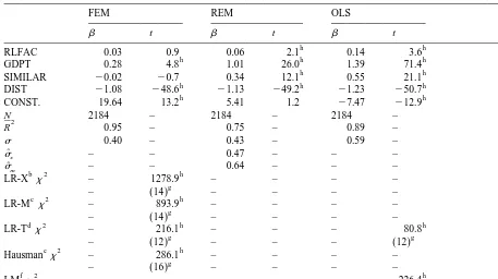
Note that the OLS estimation was shown as it had to be estimated for the Lagrange multiplier test. As we are about to test whether the country specific (export and import) effects should be modeled by a FEM and not a REM, time effects are treated as fixed for all estimations (also for OLS). From the Lagrange multiplier test statistic we see that the assumption of OLS that there is no groupwise heteroscedasticity is rejected. In the OLS and the REM estimations all the coefficients have the
6
expected sign and are highly significant. The results for the FEM emphasize that relative country size (SIMILAR) and distance in relative factor endowments (RLFAC) do not vary much in the time dimension and are captured by the country-specific fixed effects. However, in the FEM we observe no significant influence of those two variables. It should be noted that this obviously is not so for distance. In all the estimations the scaling variable (GDPT) and distance (DIST) exhibit major influence. The likelihood ratio tests in the FEM reveal that a lot of information is coming from country-effects and, thus, out of the cross-section. The restriction of time-effects to be zero is also rejected in both the OLS and the FEM estimations. The highly significant Hausman statistic in our case is driven by differences both between the variance-covariance matrices of the models and also the parameter estimates. It demonstrates that the FEM is consistent, but REM (FGLS) is not.
4. Conclusions
Most of the contributions to the empirical gravity literature made use of cross-section data. Wang and Winters (1991) and Hamilton and Winters (1992) followed this line as well as Collins and Rodrik
`
(1991). A panel framework has many advantages vis-a-vis the cross-section approach. First of all it allows to disentangle country-specific and time-specific effects. The present paper demonstrates that the proper econometric specification of a gravity model in most applications would be one of fixed
2
country and time effects. This was demonstrated by the Hausman x -test and was motivated by the explanation of country effects as widely predetermined because of geographical, historical, or political contexts.
5 ´ ´
Matyas (1998) provides a solution for the estimation of the variance components from the OLS residuals in a three-way unbalanced gravity panel model.
6
Table 1
GDPT 0.28 4.8 1.01 26.0 1.39 71.4
h h
Note: country and time effects are not reported. b
Likelihood ratio test, Greene (1997, p. 161): fixed export effects. c
Breusch–Pagan Lagrange multiplier test, Baltagi (1995), p. 62: Testing for random effects. Note, that the test was computed for the average year:
with LM5LM11LM . As we observe 12 years, the corresponding residuals and residual squares are divided by this number2 to obtain time averages. X and M are the group sizes for exporters and importers, each 14 in our case.
g
Degrees of freedom in parenthesis. h
Significant at 1%.
Acknowledgements
´ ´
Kohler, L. Matyas, and M. Pfaffermayr for helpful discussions. Of course, any remaining errors are my own.
References
Baldwin, R., 1994. In: Towards an Integrated Europe, CEPR, London. Baltagi, B., 1995. In: Econometric Analysis of Panel Data, Wiley, Chichester.
Breuss, F., Egger, P., 1998. How Reliable are Estimations of East-West Trade Potentials based on Cross-Section Gravity Analyses? Revised Working Paper, Austrian Institute of Economic Research, Vienna.
Collins, S., Rodrik, D., 1991. In: Eastern European and the Soviet Union in the World Economy, Institute of International Economics, Washington, DC.
Deardorff, A.V., 1995. Determinants of Bilateral Trade: Does Gravity Work in a Neoclassic World, NBER Working Paper 5377.
Greene, W.H., 1995. Limdep, Version 7.0, User’s Manual, Econometric Software, Bellport. Greene, W.H., 1997. In: Econometric Analysis, 3rd ed., Prentice-Hall International, London.
Hamilton, C.B., Winters, L.A., 1992. Opening up international trade with Eastern Europe. Economic Policy 14, 77–116. Helpman, E., 1987. Imperfect competition and international trade: evidence from fourteen industrial countries. Journal of the
Japanese and International Economies 1 (1), 62–81.
Helpman, E., Krugman, P.R., 1985. In: Market Structure and Foreign Trade. Increasing Returns, Imperfect Competition, and the International Economy, MIT Press, Cambridge, MA.
Hsiao, C., 1986. In: Analysis of Panel Data, Cambridge University Press, Cambridge, MA. ´ ´
Matyas, L., 1997. Proper econometric specification of the gravity model. The World Economy 20 (3), 363–368. ´ ´
Matyas, L., 1998. The Gravity Model: some econometric considerations. The World Economy 21 (3), 397–401.
Schmalensee, R., 1989. Inter-industry studies of structure and performance. In: Schmalensee, R., Willig, R.D. (Eds.), Handbook of Industrial Organization, Vol. 2, North-Holland, Amsterdam.
Schumacher, D., 1997. In: Perspektiven des Außenhandels zwischen West- und Osteuropa: Ein disaggregierter Gravitation-¨
sansatz, Deutsches Institut fur Wirtschaftsforschung, Berlin.
Wang, Z.K., Winters, L.A., 1991. The Trading Potential of Eastern Europe, CEPR Discussion Paper 610.