Non-renewability in forest rotations: implications for
economic and ecosystem sustainability
Jon D. Erickson
a,*, Duane Chapman
b, Timothy J. Fahey
c, Martin J. Christ
d aDepartment of Economics,Rensselear Polytechnic Institute,Troy,NY12180-3590,USAbDepartment of Agricultural,Resource,and Managerial Economics,Cornell Uni6ersity,Ithaca,NY14853-7801,USA cDepartment of Natural Resources,Cornell Uni6ersity,Ithaca,NY14853-7801,USA
dDepartment of Biology,West Virginia Uni6ersity,Morgantown,WV26506,USA Received 4 May 1998; received in revised form 19 March 1999; accepted 19 March 1999
Abstract
The forest rotations problem has been considered by generations of economists (Fisher, 1930; Boulding, 1966; Samuelson, 1976). Traditionally, the forest resource across all future harvest periods is assumed to grow without memory of past harvest periods. This paper integrates economic theory and intertemporal ecological mechanics, linking current harvest decisions with future forest growth, financial value, and ecosystem health. Results and implications of a non-renewable forest resource and the influence of rotation length and number on forest recovery are reported. Cost estimates of moving from short-term economic rotations to long-term ecological rotations suggest the level of incentive required for one aspect of ecosystem management. A net private cost of maintaining ecosystem health emerges and, for public policy purposes, can be compared with measures of non-timber amenity values and social benefits exhibiting increasing returns to rotation length. © 1999 Elsevier Science B.V. All rights reserved.
Keywords:Forest rotation; Ecosystem management; Ecological economic modeling
1. Introduction
Ecological economics has distinguished itself from traditional economic analysis of the
environ-ment by stressing the essential role of ecosystem services and the maintenance of ecosystem pro-cesses. Traditional analysis of renewable resources such as forests, fisheries, and agriculture has long stressed the conditions for steady-state systems of management. The economic study of these natural resources, however, has often overlooked critical intertemporal ecological mechanics related to the timing and impact of disturbing natural systems.
Based on a paper presented in a session entitled ‘Modeling Spatial and Temporal Dynamics of Terrestrial Ecosystems’, at the Fourth Biennial Meeting of the International Society for Ecological Economics, Boston University, August 4 – 7, 1996.
* Corresponding author.
E-mail address:[email protected] (J.D. Erickson)
The study of the regeneration of forests under centuries long harvest sequences is beginning to redefine our understanding of resource renewabil-ity. Traditional financial models of the forest re-source assume perfect renewability in forest growth following infinite optimal rotations of constant length. Study of forest ecology, however, suggests that rotations affect future growth, product quality, and forest health. For instance, alteration of successional sequences, nutrient cy-cles, and other components of ecosystem function are influenced by rotation length, harvest inten-sity, and cutting frequency. These cross-harvest interactions suggest a non-renewable forest growth specification, leading to the addition of a marginal benefit of recovery in the traditional optimal rotation decision rule.
In this paper, an integrated forest succession, product, and price model for the northern hard-wood forest ecosystem is developed to evaluate the impact of increasing density of pioneer species following disturbance on rotation length and tim-ber profits. For the ecosystem type examined, the success of early successional species in distur-bance – recovery cycles due to short, repetitive ro-tations have the effect of delaying forest development and entrance into late successional, higher quality, higher return species. Accordingly, an overlooked financial benefit to forest recovery is specified and estimated for a discrete horizon rotations problem. A non-renewable growth spe-cification has the effect over traditional models of lengthening forest rotations, adjusting profits downwards, and valuing the long-term mainte-nance of ecosystem processes. By incorporating ecosystem modeling into an economic framework, a clearer management picture results.
2. The marginal benefit of recovery
For the commercial forest manager, the princi-pal economic question centers on harvest timing. The majority of the economic literature on this question is grounded in the model developed in the 19th century by the German tax collector Martin Faustmann (Faustmann, 1849). Faust-mann was concerned with estimating the
bare-land expected profits1 of a forthcoming forest.
Assuming land is to remain in forestry, the prob-lem is to solve for the rotation length (T) over an infinite stream of future profits from harvesting a perfectly renewable resource.
Assuming a continuous-time discount factor (e−dt) and a continuously twice differentiable
stand profit function (p(t)), the infinite horizon profit maximization problem converges to:
Max P= p(t)
edt−1 (1)
where:
p(t)=P Q(t). (2)
Stumpage price (P) equals net price per unit volume. Natural regeneration is assumed, so re-planting costs are assumed zero. In the most general case of the multispecies, multiquality problem,Prepresents a matrix of stumpage prices and, likewise, Q(t) models a matrix of timber volumes across species and quality classes.
Solving Eq. (1) produces the following first-or-der condition, known as the Faustmann formula:
p%(t)=d p(t)+d p(t)
edt−1 (3)
From Eq. (3), a single optimal rotation length (T) maximizes net present value (P) by equating the marginal benefit of waiting to the marginal opportunity cost of delaying the harvest of the current stand (i.e. interest forgone on current profit) plus the marginal opportunity cost of de-laying the harvest of all future stands (i.e. interest forgone on all future profits, often called site value).2
1The term ‘value’ has been used to represent forest profits (e.g. Clark, 1990) in economics. Here, ‘value’ is reserved for problems incorporating non-forest amenities and other posi-tive externalities. For example, forest profits include only income from the sale of timber, where forest value would include non-market goods such as aesthics, biodiversity, or recreation.
2If real stumpage prices are assumed to grow at a rater, then the Faustmann formula simply becomes: p%(t)=(d− r)p(t)+[(d−r)p(t)]/[e(d−r)t−1]. Eqs. (29) – (33) in the
Fig. 1. Cubic forest undiscounted profit functions.
Adaptations and expansions to this model in-clude modeling non-timber benefits (e.g. Hart-man, 1976; Calish et al., 1978; Berck, 1981), multiple-use forestry (e.g. Bowes and Krutilla, 1989; Snyder and Bhattacharyya, 1990; Swallow and Wear, 1993), stochastic price paths (e.g. Clarke and Reed, 1989; Forboseh et al., 1996), market structure (e.g. Crabbe and Van Long, 1989), and uneven aged forestry (e.g. Mont-gomery and Adams, 1995).
All these improvements to the basic Faustmann formula, however, share a strong assumption of perfect growth renewability — a constant growth function (Q(T)) across all future planning peri-ods. In contrast, evidence from the study of forest ecology and management indicates a strong rela-tionship between rotation length, rotation fre-quency, and harvest magnitude in a current management period, with the growth and mainte-nance of the forest in future periods (e.g. Borman and Likens, 1979; Kimmins, 1987). This is partic-ularly the case where natural regeneration seeds the new forest, or soil renewability is compro-mised. In the Faustmann framework, this ecologi-cal knowledge implies a forest stand profit function dependent on rotation length (T) and rotation number (i), given constant technology and harvest magnitude.
Growth in merchantable timber volume is typi-cally modeled using a cubic or exponential form,
consistent with stages for rapid growth, biological maturity, and disease and decay (Clark, 1990). Consider a cubic functional form for undis-counted profit at constant prices:
p(t)=b1t+b2t2+b3t3. (4)
Fig. 1 illustrates three plots of Eq. (4) following a harvest at T0 assuming different parameter val-ues forb1,b2, andb3. SupposeT1A is an optimal
Faustmann rotation in the first harvest cycle (i= 1). Therefore, a longer rotation in this first cycle (for instance, T1B) would be sub-optimal as it would decrease the marginal value of waiting below the sum of first harvest and future harvest opportunity costs.
However, there may be an additional marginal variable to consider in the first rotation decision. Suppose rotation length in the first harvest cycle influences the form of the functional stand profit function in subsequent cycles. For instance, sup-pose the choice of T1Ain cyclei=1 results in the profit function p(Ti=2T1A) in cycle i=2. A
longer rotation such as T1B, however, results in a higher profit function p(Ti=2T1B) in cycle i=2.
In this case, a longer first rotation has the benefit of allowing the forest more time to recover from the initial cut at T0. Now, waiting until T1B to
harvest during the first cycle has the benefit of shifting the second cycle curve upwards to p(Ti=
result in an identical second rotation profit function. Without taking into account this cross-harvest impact, the Faustmann solution ofT1Awould lead
to a sub-optimal decision.
To incorporate this interaction between current harvest length and subsequent profit functions consider Eq. (5). The function f(Ti−1,i−1) is
added as a variable to the periodiprofit function. The level of f(Ti−1,i−1), or ecological impact,
depends on the length of the last period’s rotation (Ti−1), and the number of rotations since the first
cut at T0 to take into account any cumulative impacts. It influences the cubic function parameters (b1,b2, andb3) of the stand profit function through
an ecological impact represented by the parameters
a1, a2, and a3:
Stand profit in the current rotation cycle (i) now depends on the current rotation length (Ti), the previous rotation length (Ti−1), and the number of
rotations (i−1) since the pre-disturbance period (i−1=0). The ecological impact function, f(), represents a forest recovery relationship based on
physical and biological parameters. For example,
f() might measure the impact on forest regeneration from pioneer species rebound (stems/acre), from soil nutrient loss (nutrients/m2) or erosion (soil
depth), or possibly from a general index of resource renewability.
The first-order conditions forf() imply that as the previous period rotation length (Ti−1) increases, the
negative ecological impact decreases. Also, as the number of rotations since the pre-disturbance pe-riod (i−1=0) increases, the ecological impact increases. An initial condition (V) is assumed which defines the level off() following the initial harvest at T0. This parameter can be considered a forest health endowment left from the previous land manager. In the case of inheriting a mature forest not previously managed,Vcould be considered the ecological effect on forest growth from periodic natural disturbances (e.g. wind storms, fires).
Assuming this non-renewable, rotation length-dependent, stand profit specification over an infinite horizon, the profit maximization problem becomes:
Max
P=p(t1,f(T0, 0))e−dT1+p(t2,f(T1, 1)) e−dT2
+p(t3,f(T2,2))e−dT3+ . . . (15)
Under an assumption of perfect renewability,
f(T0, 0)=f(T1, 1)=. . .=f(T,)=V, and the
profit maximization problem converges to Eq. (1), from which the usual Faustmann result of a con-stant rotation length in Eq. (3) is obtained.
Under the assumption of partial non-renewabil-ity, however, the selection of the optimal rotation length set (Tifori=1, 2, 3, . . .) now considers the impact on each subsequent period’s profits through the addition of a marginal benefit of recovery (MBR). The marginal benefit of recovery in period
ifrom a rotation length in the previous periodi−1 is represented as:
Fig. 2. Kimmins’ ecological rotation vs. successional retrogression (Kimmins, 1987).
In the forest ecology literature, Kimmins (1987) outlines the distinction between a Faustmann-type rotation where net present value is maximized, and an ecological rotation, the time required for a site managed with a given technology to return to the pre-disturbance ecological condition. Fig. 2 demonstrates the concept of an ecological rota-tion, and the hypothetical case of rotating before a successional sequence is completed. Succession is defined as the orderly replacement over time of one species or community of species by another, resulting from competitive interactions between them for limited site resources (Marchand, 1987). The vertical axis of Fig. 2 delineates a range from early successional species (pioneer) to late succes-sional species (climax).
Under a moderate disturbance regime (for in-stance, stem harvesting or selective cutting),Tand 2T represent two Faustmann rotations. The de-clining path of ‘backwards’ succession is referred to as successional retrogression. For a moderate disturbance, an ecological rotation is represented by Te, the time when the forest recovers to the
original successional condition. A more severe disturbance regime (for instance, whole-tree har-vesting or clear-cutting) is also represented where
a longer ecological rotation (TE) would
necessar-ily be required for successional rebound. Ecologi-cal observations also suggest the possibility that severe or repeated disturbance could shift the biotic community into a different domain in which the mature (climax) phase of succession is very different than the pre-disturbance condition (Perry et al., 1989). For instance, a clear-cut of a mature forest resulting in the permanent replace-ment by grasslands might be represented in Fig. 2 as a path that never rebounds.
While Fig. 2 focuses on a potential decay in successional pathways due to short forest rota-tions, a similar diagram could model other ecosys-tem retrogressions. For example, Federer et al. (1989) describe the effects of intensive harvest on the long-term soil depletion of calcium and other nutrients, and the potential limiting effect on forest growth.
deci-sions, with both economic and ecological benefits. Furthermore, valuing ecosystem recovery may benefit non-timber amenities exhibiting increasing returns inTas described elsewhere (often referred to as the Hartman model after Hartman, 1976). Lastly, the cost and benefits of moving from economic rotations to ecological rotations can be obtained and used for public policy extensions.
3. An ecological economic model of the northern hardwood forest
The northern hardwood forest ecosystem is the dominant hardwood component of the larger northern forest of the United States, stretching west to northern Minnesota, east through New England, south into parts of the Pennsylvania Appalachians, and north into Canada. It is char-acterized by sugar maple (Acer saccharum), American beech (Fagus grandifolia), and yellow birch (Betula alleghaniensis) predominance, with varying admixtures of other hardwoods and soft-woods. A model was developed to account for forest growth, pioneer species introduction, con-version from biomass to merchantable timber and pulpwood, and stumpage price growth. Develop-ment and details of these four components are described in detail in Erickson et al. (1997).
3.1. Growth simulation
The stochastic forest growth simulator JABOWA developed by Christ et al. (1995) was used to model succession and growth following a clear-cut in the northern hardwood forest. The JABOWA model simulates growth of individual trees on small plots at the forest gap level, built on silvical data for the species of the Hubbard Brook Experimental Forest in the White Moun-tains of New Hampshire. ‘Gap’ refers to a hole in the forest canopy created by the felling of a tree, naturally or otherwise. Christ et al. (1995) devel-oped a version of the model in PASCAL to test the accuracy of the original Botkin et al. (1972) model predictions against forest inventory data. Model development, parameters, and forest spe-cies characteristics are described in Erickson et al.
(1997). In general, growth algorithms for each species consist of the following components (adapted from Botkin et al., 1972):
Dd=G(s, L, dmax, hmax) ·r(L(I, Z))
·h(D, Dmin,Dmax) ·S(A,u) (17)
G()=sL{1−[(d·h)/(dmax·hmax)]} (18)
r()=1−e−4.64(L−0.05) {shade-tolerant} (19)
r()=2.24 (1−e−1.136(L−0.08)) {shade-intolerant}
(20)
where:
L=Ie−kZ (21)
h()=4(D−Dmin)(Dmax−D)
(Dmax−Dmin)2 (22)
S()=1−A/u (23)
Eq. (17) represents the annual change in species diameter at breast height (d). Only growth in diameter is modeled because it will be used to predict merchantable volume (Q) by species and product class for estimating the stand profit func-tion in Eq. (1). The funcfunc-tion G represents a growth rate equation for each species under opti-mal conditions, depending on a solar energy uti-lization factor (s), leaf area (L), and maximum values for diameter (dmax) and height (hmax).
The remaining right-hand side functions act as multipliers to the optimal growth function to take into account shading, climate, and soil quality. The shading function, r, is modeled separately for shatolerant and -intolerant species and de-pends on available light to the tree (a function of annual insolation (I) and shading leaf area (Z)). The functionhaccounts for the effect of tempera-ture on photosynthetic rates, and depends on the number of growing degree-days (D) and species specific minimum and maximum values of D for which growth is possible. Lastly, S is a dynamic soil quality index dependent on total basal area (A) on the plot and maximum basal area (u) under optimal growing conditions.
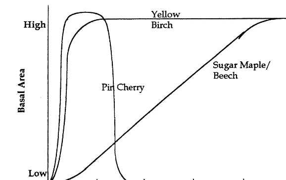
Fig. 3. Northern hardwood succession following clear-cut.
die. Species characteristics and chance determine the dynamics of these birth – growth – death cycles. New saplings randomly enter the plot within lim-its imposed by their relative shade tolerance and degree-day and soil moisture requirements. As taller trees shade smaller ones, the amount of shading is dependent on the species’ characteristic leaf number and area, and survival under shaded conditions depends on the shade tolerance of a species. Given this stochasticity, simulation data vary widely with each model run.3
3.2. Successional retrogression
Building on the JABOWA model, the challenge is to incorporate an ecological mechanism to cap-ture Kimmins’ hypothesis of rotation-dependent succession and growth. Such a mechanism is evi-dent in the early succession rebound of pioneer species. A possible succession of dominant species is represented by Fig. 3, adapted from Marks (1974).
During the first 15 – 20 years following a clear-cut, the recovering forest is dominated by pioneer
species such as raspberry bushes, birches, and pin cherry. These fast growing, opportunistic species play a critical role in ecosystem recovery from a clear-cut by reducing run-off and limiting soil and nutrient loss (Marks, 1974). However, their initial density will also influence stand biomass accumu-lation and growth of commercial species (Wilson and Jenson, 1954; Marquis, 1969; Mou et al., 1993; Heitzman and Nyland, 1994).
In this application to the northern hardwood forest, pin cherry (Prunus pensyl6anica) is
as-sumed to be the dominant pioneer species. As a particularly fast growing, short-lived, shade-intol-erant species with no commercial value, the effect of its growth following a clear-cut on forest suc-cession and future harvest profits can be signifi-cant. Tierney and Fahey (1998) demonstrate the influence of short rotations on the survival of its seeds, and its subsequent germination and growth at very high density in young stands. This forest ecology research indicates that pioneer species densities may stabilize at low levels following a 120-year or more rotation regime (comparable with a Kimmins’ ecological rotation). Rotations at 60-year intervals (closer to a Faustmann eco-nomic rotation) result in increasing pioneer spe-cies densities toward a carrying capacity asymptote.
The dependence of the initial density of a pio-neer species (PS) on the previous harvest rotation length (Ti−1) and the number of previous harvests
(i−1) is used to represent the more general case of successional retrogression from Fig. 2. The following ordinary least squares model was esti-mated to capture the hypothesis of a rotation-de-pendent ecological impact function proposed in Eq. (5). Estimation is based on data from the soil seed bank dynamic modeling results of Tierney and Fahey (1998). Ecological assumptions and research results are reported in Erickson et al. (1997).
3.3. Multiproduct, stochastic quality model
The third model component converts biomass output from JABOWA into economic output. The financial value of standing timber depends on age, size, species, and quality distributions. A typical northern hardwood stand can provide sawtimber, pulpwood, and firewood. Depending on the market and the land owners motivations, any combination of these three product classes may be managed. Stand profit is represented as5:
P(t, PS)=
!
% given initial pioneer species density (PS). Pioneer species density influences profitability throughin-troducing significant competition for light and other resourcs in the JABOWA model during early stand development. As in Eq. (1), total stand profit (US$/acre) is the product of a price matrix (Pt) and merchantable volume (Q) for
eight commercial species (S=1 – 8) and a non-commercial species group (S=9) in each product category (C=1 – 6). Product categories are com-prised of grade 1 – 3 timber (C=1 – 3), below grade sawtimber (C=4), and hardwood (C=5) and softwood (C=6) pulp. To assign quality classes, a random number is generated and as-signed to each stem and compared with class probability limits as estimated by a generalized logistic regression (GLR) model developed by Yaussy (1993). The GLR procedure, parameters, and an example are described in Erickson et al. (1997). Firewood output was not considered.
Merchantable volume (Q) is modeled on stem diameter (d), provided for each tree by a growth simulation, and merchantable length (M), which is also modeled on d. The level of initial pioneer species density (PS) is predicted from Eq. (25) based on the previous period’s rotation length (Ti−1) and number (i−1). PS influences diameter
growth through the dynamics of the forest growth simulator, as well as influencing merchantable volume calculations through impacting forest site quality. The procedures for converting diameter estimates to merchantable volume by species and product class are described in detail in Erickson et al. (1997).
3.4. Parameterization
Integrating the first three components of the model outlined above, merchantable stand vol-umes were generated at 10-year intervals from year 20 to 250, at initial pioneer species densities of 0, 10, 20, 50, 100, 200, 500, 1000, 2000, and 5000 stems per 100 m2. Volume within each
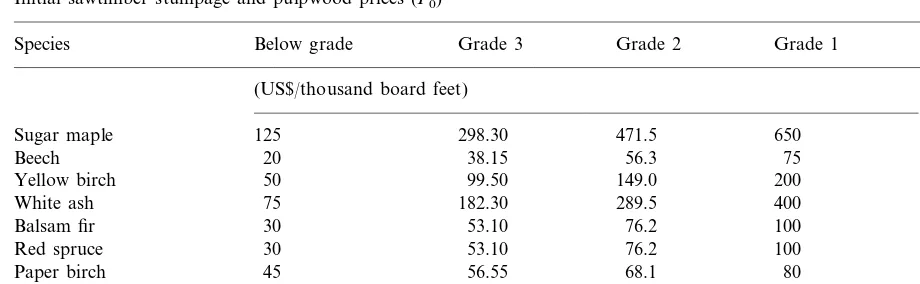
spe-cies, product class, and year was then converted to profit by multiplying a net price matrix of 1995 stumpage prices. The initial distribution of net prices (P0) across product classes and species is summarized in Table 1. Stand profit for each year was then summarized across all products and species to generate data for p(t, PS) at each PS value run.
4All parameters are significant ata=0.10; R2=0.98;F= 65.05.
650
Sugar maple 125 298.30 471.5 7
75
Beech 20 38.15 56.3 7
200 7
Yellow birch 50 99.50 149.0
289.5 400 7
White ash 75 182.30
100
Balsam fir 30 53.10 76.2 12
100 12
Red spruce 30 53.10 76.2
68.1 80
Paper birch 45 56.55 7
7 150
Red maple 50 83.00 116.0
–
Non-commercial – – – 7
aNote: Sawtimber prices in each quality class were calculated from ranges of stumpage prices reported in NYDEC (1995) for the Adirondack region. Within each range: min=below grade price, 33rd percentile=grade 3 price, 66th percentile=grade 2 price, and max=grade 1 price.
This specification results in a 264×6 explana-tory variable matrix. The following cubic model was fitted6:
p(t, PS)=(b1+a1PS)t+(b2+a2PS2)t2
+(b3+a3PS)t3 (27)
p(t, PS)
=(7.718−0.0025PS)t
+(0.219+1.52×10⁻⁹PS2) t2
−(0.00082+1.40×10⁻⁸PS)
t3. (28)
Fig. 4 plots p() at some illustrative PS values. Here p() represents stand profit at 1995 prices. Price growth is taken up separately in Section 3.5.
3.5. Price growth(Pt)
The influences on stumpage prices at the forest stand level are complex. They might include: tim-ber quality, volume to be cut per acre, logging terrain, market demand, distance to market, sea-son of year, distance to public roads, woods labor costs, size of the average tree to be cut, type of logging equipment, percentage of timber species in the area, end product of manufacture, landowner requirements, landowner knowledge of
market value, property taxes, performance bond requirements, and insurance costs (NYDEC, 1995). At the macroeconomic level, exports, mill stocks, and aggregate demand are typically ex-planatory variables (Luppold and Jacobsen, 1985). Emerging effects on northeast stumpage prices include increasing substitution of recycled fibers in paper making, board feet restrictions on removals in the Northwestern United States, and continued growth in global wood demand.
For the purposes of this model, the Pt matrix
will depend on an initial price distribution att=0 (see Table 1), and algorithms for growth in three product classes. As a stand matures, it is assumed to enter three stages of product development: (1) pulpwood, (2) low quality sawtimber, and (3) high quality sawtimber. To illustrate, Fig. 5 plots a representative model run. Here prices are assumed
Fig. 4.p(T, PS) at five initial pioneer species (PS) densities. 6Assessment:a
1,b2,a2, andb3all significant ataB0.005;
b1 and a3 significant at a=0.073 and 0.209, respectively;
Fig. 5. Sugar maple stumpage and hardwood pulp value, PS=0, 1995 US$/acre.
an exponential growth rate of r(t)=1%. At tL, the stand shifts into a low quality sawtimber phase (below grade and grade 3), and the expo-nential growth rate increases to 3%. As the stand continues to mature, high quality timber becomes more prevalent until a time tH is
reached when timber prices grow at a maximum rate more characteristic of high quality timber.
As continued short rotations enhance pioneer species abundance, species competition pushes commercial species development further into the future, thus delaying the entrance into higher quality product classes. To capture this succes-sional retrogression hypothesis, a shift variable (Di) is assumed to add years to tL and tH
de-pending on pioneer species density at the begin-ning of each rotation.
This model is applied by mapping three expo-nential growth functions over the planning hori-zon at each rate. The function is applied as a multiplier to the initial species by product price matrix (P0), with r depending on t.
4. Rotation analysis
With the non-renewable stand value specifica-tion of Eq. (28) and the price growth model assumed in Eqs. (29) – (33), the analysis turns to estimating and comparing rotation lengths. Spe-cifically, the question of whether the benefits from recovery in future harvest periods influence the harvest timing decision in current periods is addressed. Four harvest cycles are modeled. A positive discount rate causes profits from harvest cycles beyond four periods to have a negligible effect on the choice of rotation lengths in earlier periods.
The applied problem is to choose the rotation set that maximizes the present value of profits over four harvest cycles. Again, timber cutting costs are reflected in the stumpage price paid to the forest owner. High labor costs are also as-sumed to prohibit thinning pioneer species from young dense stands. This can be solved as a four-stage dynamic programming problem. to remain constant over a 250-year horizon, no
additional pioneer species are added, and only sugar maple and total hardwood pulpwood val-ues are plotted. Initially the stand generates mostly hardwood pulpwood. Below grade sugar maple sawtimber rises steadily over time, sur-passed first by grade 3 lumber, and eventually by grade 2 and 1 as the stand matures.
To capture these dynamics, an exponential model for stand profit growth with a shifting growth rate is assumed. In the northeastern US, from 1961 – 1991, Sendak (1994) reports average real hardwood stumpage prices for sawtimber rose 4.3% per year, and for pulpwood rose 1.3% per year. As these rates are an average across all quality classes and species, the following price growth model is assumed to apply to the entire price matrix:
Pt=P0er(t)t (29)
where:
r(t)=1% if t5tL+DI (30)
r(t)=3% if tL+DiBt5tH+DI (31)
r(t)=4% if t\tH+DI (32)
and
DI=PS/250 (33)
+e
r(T2)(T1+T2)p(T2,f(T1, 1))
ed(T1+T2) +…
+e
r(T4)(T1+T2+T3+T4)p(T4,f(T3, 3))
ed(T1+T2+T3+T4) (34)
Max
P=e(r(T1)−d)T1p(T1, PS 0)
+e(r(T2)−d)(T1+T2)p(T2,f(T1, 1))+…
+e(r(T4)−d)(T1+T2+T3+T4)p(T4,f(T3, 3)) (35)
4.1. Risk and choosing an economic optimum
The difficulty in solving Eq. (35) over four periods is that asrvaries within each rotation cycle (from 1 to 3 to 4%), the possibility of multiple optimums arises. To illustrate, take the case of maximizing profit over a single rotation. Assuming PS=100,d=5%,tL=30, andtH=100, two local optimums emerge, at T=70 andT=196. Under the model assumptions, a 196-year global optimum stabilizes the pioneer species seed bank at ‘natural’ background levels, and thus the profit-maximizing single rotation is potentially a Kimmins’ ecological rotation.
However, is this a realistic rotation length? Indeed, at a discount rate of 5% a rotation length ofT=70 is perhaps more characteristic of the end of most commercial rotations for large landowners in the northern hardwood forest.
Are managers behaving irrationally? Not when risk and uncertainty are taken into account. A landholder will not face a profit maximization problem with perfectly forecasted profits. Risk and uncertainty increase in later periods through mar-ket, government, and environmental variability. For example, as a forest matures its potential for yielding high quality wood increases, but so does the likelihood of disease, aging effects, or blow-down. Furthermore, given the public’s preference for old growth forests, there may be a risk of stricter cutting regulations as a stand ages. As present value
of simply raising the landowner’s discount rate in the high quality timber phase (T\100 years) by two percentage points.7 One optimum at T=70
results. A product phase-dependent discount rate has some intuitive appeal, and is helpful in solving the multirotation problem.
4.2. The optimal rotation set with risk, and the marginal benefit of reco6ery
Assume that because of risk and uncertainty the hypothetical landowner will maximize profits in either the low quality timber or pulpwood price phases. The task is to solve Eq. (35) forT1,T2,T3
and T4. Parameter values are as follows: d=5%, PS0=100, tL=30, and tH=100.
Table 2 outlines the optimal rotation set under two cases. The first is the successional retrogression hypothesis withp(Ti,f(Ti−1,i−1)). The second is
the traditional perfectly renewable growth
hypoth-Table 2
Four harvest period solution with 2% long-run risk factor Renewable growth Rotation-dependent
Rotation
specification mis-specification
p(TN,f(TN−1,N p(TN, PSN=100) −1)
Years
T1 58 40
68
T2 44
51
T3 70
83 70
T4
US$400.3/acre US$470.2/acre Net present
value
esis with p(Ti, PSi=100). The sum of present
value over four periods reveals a 17.5% overesti-mate of stand profits in the traditional specifica-tion. Rotation lengths differ by as much as 24 years in the second cycle, and become longer in future cycles as prices continue to grow exponen-tially and profit from future rotations goes to zero. The rotation length forT4simply maximizes profits in this cycle.
Compare the first cycle rotation lengths with that of the single rotation problem, where T
equaled 70 years. The effect of considering profits in cycles 2, 3 and 4 at considerably higher prices and identical growth conditions reduces T1 from 70 to 40 years. This is the result of considering three period future profits. When successional ret-rogression is assumed, the shift from 40 to 58 years is the result of including a marginal benefit of recovery.
Differentiating Eq. (35) byT1yields the first-or-der condition for T1. The terms can be arranged so the marginal benefit of waiting another period equals the marginal cost of delaying first cycle profits plus the marginal cost of delaying all fu-ture profits (site value), as was the case in the traditional Faustmann formula, and the addition of a marginal benefit of recovery in the second cycle:
At the optimal first cycle rotation (T1=58) the
marginal benefit of waiting another year until harvest is US$7.50. It equals the marginal cost of delaying first cycle profits of US$6.30, the
mar-Table 3
The optimal four-cycle rotation set and long-run economic and ecological health, varying the discount rate
d(%)
Net present valueb
1592 500 Undiscounted profit @ year 105b 5909
Ecological indicators
ginal cost of delaying the next three harvests (site value) of US$1.70, and the marginal benefit of recovery in future cycles of US$0.50. Site value well exceeds MBR because of the effect of expo-nential price growth.
4.3. Economic and ecological indicators under 6arious discount rates
with a total present value of US$24/acre. At
d=10% the optimal rotation set occurs in the low quality sawtimber phase at rotations of 31, 51, 48 and 51 years, all of which are corner solutions since tL=30, D1=21, D2=18 and D3=21. At d=5%, the solution occurs at the corner of the high quality sawtimber phase.
The sum of present value over four cycles indi-cates the effect on profit of both shorter rotations with lower quality products and a higher discount rate. A second economic indicator, summarizing stand profit at year 105 (the end of the fourth cycle under d=15%) with no discounting, indi-cates only the effect of shorter rotations and lower quality products on future profits. Under this second indication, just over one rotation of high quality sawtimber (at T1=101 and T2=4) produces 2.7 times more undiscounted profits than three and a half rotations under the low quality management case, and 10.8 times more undiscounted profits than four full pulpwood rotations.
The ecological indicators of the three manage-ment scenarios reflect the important ecological benefits to longer rotations. At the beginning of the fourth harvest cycle, pioneer species density is 2224 stems under long rotations, 5277 stems un-der medium length rotations, and 6538 stems under short rotations. In the pulpwood harvesting case, entrance into both sawtimber phases is de-layed a full 27 years by the fourth harvest cycle. The cases where d=10% and d=15% demon-strate the declining trend in successional integrity as suggested by the Kimmins’ successional retro-gression hypothesis, while the case where d=5% perhaps approaches a set of ecological rotations (i.e. both scenarios outlined in Fig. 2).
4.4. Single period management under declining forest health
Another method to solving the multiple rota-tions problem is to assume the values for PSiover
Here, the first-order condition within each cycle becomes:
d−r(T1)=p%(Ti, PSi−1)
p(Ti, PSi−1)
(40)
Again, assuming the landowner will manage either in the low quality sawtimber or pulpwood price growth phases, the four-cycle interior solu-tion for Tis 70, 80, 80, and 83. Future landown-ers must wait longer to maximize profits due to poorer forest health endowments. Profits continue to increase in later cycles due to exponential price growth, however, timber quality and quantity are constrained by a degrading resource. By the fourth cycle, the pulpwood price phase is 70 years long, and initial pioneer species density is 3979 stems/acre.
4.5. Ecological rotations and 6aluing non-timber amenities
As was evident in the single period problem, given low constant discount rates ecological rota-tions may be economically optimal. Solving Eq. (35) with a constant discount rate of 5% yielded the rotation length set of 101, 107, 108 and 115 years with a total present value of US$1122.6/ acre. Assuming constant initial pioneer species density across all future harvest cycles (i.e. PS= 100 andDi=0), the optimal set becomes 101, 101,
101 and 116 with a total present value of US$1200.2/acre. Not accounting for non-re-newability results in a negligible 2% overestimate of total present value.
Perhaps including the value of non-timber amenities would justify ecological rotation lengths as socially optimal. Amenity values that exhibit increasing returns to rotation length might include recreation value, provision for certain habitats, and watershed protection. For example, referring to Table 3, consider the low discount rate solution (d=5%) and middle discount rate solution (d= 10%) as the social and private optimal rotation sets. Next, evaluating the social rotation set at the private discount rate of 10% results in a total present value of just US$5/acre. If a landowner was forced to rotate at these lengths, this would result in a private loss of US$41/acre. However, if the sum of non-timber amenities exceeds this loss and the landowner experiences these benefits di-rectly (for example, hunting or recreational use), then there may be a private incentive to lengthen rotations.
Alternatively, if the amenity values are of a strictly social nature (for example, watershed pro-tection or biodiversity preservation) then an op-portunity may exist for the government or an environmental group to accommodate the land owner’s loss in timber profits through a payment or incentive mechanism (for example, paying for a conservation easement or providing tax relief). In addition, alternative silviculture practices such as selective cutting may strike common ground be-tween the interplay of social and private benefits. Furthermore, assessing the ecological impact of economic decisions contributes to the definition and assessment of ‘new’ or ‘sustainable’ forestry, which embraces management practices derived from ecological principles (Franklin, 1989; Gillis, 1990; Gane, 1992; Fiedler, 1992; Maser, 1994).
5. Concluding remarks
Accounting for the ecological recovery of the northern hardwood forest over a series of harvests was shown to increase rotation lengths over the traditional Faustmann result. A positive marginal benefit of recovery offsets the marginal costs of delaying current and future rotations, creating a benefit to delaying rotations under a non-renew-able stand value growth specification.
The model presented in this paper is limited to the specific ecological dynamic of pioneer species introduction and interspecies competition for light and other resources. In the context of forest man-agement, this approach can be generalized to many intertemporal dynamics such as other suc-cessional sequences, alteration of nutrient cycles, or disturbance from anthropogenic climate change. Knowledge of benefits to ecosystem re-covery can help define both ecological and eco-nomic rotation lengths under various scenarios of Kimmins’ ecosystem retrogression. At one ex-treme, given low discount rates and risk, relatively long ecological rotations may be economically optimal. At the other extreme, a site managed with short rotations motivated by short-term profits and a high discount rate may result in degraded forest stands with low value species — a detriment to long-run ecological health and social benefits.
When considering social welfare and the maintenance of ecosystem processes from multi-ple-use management, many non-timber benefits have increasing returns in rotation length and decreasing returns to harvest intensity. The benefit of recovery was shown to have a market value, and its inclusion more accurately estimates the optimal rotation set. Including this benefit, how-ever, may not completely provide the private in-centive to move from ecologically unsustainable to sustainable rotation lengths and practices, par-ticularly when the net private cost of doing so is high. However, this net private cost can be com-pared with benefits from non-timber amenities and alternative management practices, or to costs of forest maintenance (i.e. thinning undesirable species), providing rationale for social management.
Acknowledgements
The authors would like to thank Jon Conrad, Bill Schultze, Neha Khanna and three reviewers for invaluable comments and suggestions.
References
Berck, P., 1981. Optimal management of renewable resources with growing demand and stock externalities. J. Environ. Econ. Manag. 8, 105 – 117.
Borman, F.H., Likens, G.E., 1979. Pattern and Process in a Forested Ecosystem: Disturbance, Development, and the Steady State Based on the Hubbard Brook Ecosystem Study. Springer-Verlag, New York, NY.
Botkin, D.B., Janak, J.F., Wallis, J.R., 1972. Some ecological consequences of a computer model of forest growth. J. Ecol. 60, 948 – 972.
Bowes, M.D., Krutilla, J.V., 1989. Multiple-Use Management: The Economics of Public Forestlands. Resources for the Future, Washington, DC.
Calish, S., Fight, R.D., Teeguarden, D.E., 1978. How do nontimber values affect Douglas-Fir rotations? J. For. 76, 217 – 221.
Christ, M., Siccama, T.G., Botkin, D.B., Borman, F.H., 1995. Comparison of stand-dynamics at the Hubbard Brook Experimental Forest, New Hampshire, with predictions of JABOWA and other forest-growth simulators. Institute of Ecosystem Studies, Millbrook, NY (Available from authors).
Clark, C.W., 1990. Mathematical Bioeconomics: the Optimal Management of Renewable Resources. John Wiley and Sons, New York, NY.
Clarke, H.R., Reed, W.J., 1989. The tree-cutting problem in a stochastic environment: the case of age-dependent growth. J. Econ. Dyn. Control 13, 569 – 595.
Crabbe, P.H., Van Long, N., 1989. Optimal forest rotation under monopoly and competition. J. Environ. Econ. Manag. 17, 54 – 65.
Erickson, J.D., Chapman, D., Fahey, T.J., Christ, M.J., 1997. Nonrenewability in forest rotations: implications for eco-nomic and ecosystem sustainability. Cornell University, Working Paper Series in Environmental and Resource Economics, 97-01, 1 – 51.
Faustmann, M., 1849. On the determination of the value which forest land and immature stands possess for forestry.
ron. Manag. 13 (5), 593 – 601.
Fiedler, C., 1992. New forestry: concepts and applications. West. Wildlands 17 (4), 2 – 7.
Forboseh, P.F., Brazee, R.J., Pickens, J.B., 1996. A strategy for multiproduct stand management with uncertain future prices. For. Sci. 42 (1), 58 – 66.
Franklin, J., 1989. Toward a new forestry. American Forests (Nov./Dec.).
Gane, M., 1992. Sustainable forestry. Commonw. For. Rev. 71 (2), 83 – 90.
Gillis, A.M., 1990. The new forestry: an ecosystem approach to land management. Bioscience 40 (8), 558 – 562. Hartman, R., 1976. The harvesting decision when a standing
forest has value. Econ. Inq. 4, 52 – 58.
Heitzman, E., Nyland, R.D., 1994. Influences of Pin Cherry (Prunus pensyl6anicaL. f.) on growth and development of young even-aged Northern Hardwoods. For. Ecol. Manag. 67, 39 – 48.
Kimmins, J.P., 1987. Forest Ecology. Macmillan, New York, NY.
Luppold, W.G., Jacobsen, J.M., 1985. The determinants of hardwood lumber price. Research Paper NE-558, USDA Forest Service, Northeastern Forest Experiment Station, Broomall, PA.
Marchand, P.J., 1987. North Woods: an Inside Look at the Nature of Forests in the Northeast. Appalachian Moun-tain Club, Boston, MA.
Marks, P.L., 1974. The role of Pin Cherry (Prunus pensyl -6anica L.) in the maintenance of stability in Northern Hardwood ecosystems. Ecol. Monogr. 44 (1), 73 – 88. Marquis, D.A. 1969. ‘Thinning in Young Northern
Hard-woods: 5 year results’. Research Paper 139, USDA Forest Service, Northeast Forest Experiment Station, Broomall, PA.
Maser, C., 1994. Sustainable Forestry: Philosophy, Science, and Economics. St. Lucie Press, Delray Beach, FL. Miner, C.L., Walters, N.R., Belli, M.L., 1988. A guide to the
TWIGS program for the North Central United States. General Technical Report NC-125, USDA Forest Service, North Central Forest Experiment Station, St. Paul, MN. Montgomery, C.A., Adams, D.M., 1995. Optimal timber
man-agement policies. In: Bromley, D.W. (Ed.), The Handbook of Environmental Economics. Blackwell, Oxford, UK. Mou, P., Fahey, T.J., Hughes, J.W., 1993. Effects of soil
disturbance on vegetation recovery and nutrient accumula-tion following whole-tree harvest of a Northern Hardwood ecosystem, HBEF. J. Appl. Ecol. 30, 661 – 675.
Perry, D.A., Amaranthus, M.P., Borchers, J.G., Borchers, S.L., Brainerd, R.E., 1989. Bootstrapping in ecosystems. Bioscience 39 (4), 230 – 237.
Sendak, P.E., 1994. Northeastern regional timber stumpage prices: 1961 – 91. Research Paper NE-683, USDA Forest Service, Northeastern Forest Experiment Station, Rad-nor, PA.
Snyder, D.L., Bhattacharyya, R.N., 1990. A more general dynamic economic model of the optimal rotation of multiple-use forests. J. Environ. Econ. Manag. 18, 168 – 175.
Swallow, S.K., Wear, D.N., 1993. Spatial interactions in multiple-use forestry and substitution and wealth effects
for the single stand. J. Environ. Econ. Manag. 25, 103 – 120.
Tierney, G.L., Fahey, T.J., 1998. Soil seed bank dynamics of Pin Cherry in northern hardwood forest, New Hamp-shire, USA. Can. J. For. Res. 28, 1471 – 1480.
Wilson, R.W., Jenson, V.S., 1954. Regeneration after clear-cutting second-growth Northern Hardwoods. Station Note 27, USDA Forest Service, Northern Forest Experi-ment Station, Radnor, PA.
Yaussy, D.A., 1993. Method for estimating potential tree-grade distributions for Northeastern forest species. Re-search Paper NE-670, USDA Forest Service, Northeastern Forest Experiment Station, Radnor, PA.