Vol. 44 (2001) 295–314
Endogenous labor supply, growth and
overlapping generations
Gilles Duranton
∗Department of Geography and Environment, London School of Economics and Political Science, Houghton Street, London WC2A 2AE, UK
Received 8 December 1998; received in revised form 6 July 2000; accepted 7 July 2000
Abstract
This paper explores a simple model of endogenous growth in an overlapping generations frame-work when labor supply is made endogenous. The following results are obtained:
• If leisure and consumption are substitutes, the economy can experience multiple equilibrium paths (including high growth and high labor supply or no growth and low labor supply). • If the demand for leisure is inelastic, then the economy enjoys steady growth as in standard
models.
• If leisure and consumption are complements, then production remains bounded, although en-dogenous growth is possible and socially desirable.
© 2001 Elsevier Science B.V. All rights reserved.
JEL classification:J22; O10; O41
Keywords:Labor supply; Growth; Overlapping generations
In the light of our earlier discussion, technological and other limitations on the supply side can hardly be viewed as an important factor. [. . .] A long term rise in real income per capita would make leisure an increasingly preferred good as is clearly evidenced by the marked reduction in the working week in freely organized non-authoritarian advanced countries. [. . .] The pressure on the demand side for further increase is likely to slacken.
Kuznets (1959)
∗Tel.:+44-171-955-7604.
E-mail address:[email protected] (G. Duranton).
1. Introduction
Although modern theories of growth tend to focus primarily on technological change, human capital, knowledge and capital accumulation, many popular explanations often relate the wealth of nations to the supply of labor. Two popular arguments are used to account for two different phenomena: the persistence of under-development in less developed countries and the slowdown of growth in the developed economies. Some countries, supposedly, remain poor because their populations are “lazy” and more subtly, rich countries do not grow as fast as they used to because of “declining efforts” of the labor force. What credit should we give to these arguments? The answer on the face of it is: not much. Of course, one can always introduce a cultural parameter to explain differences in labor supply but the causality that goes from laziness to poverty is probably at best spurious. The most obvious counter-example is that this type of view attributed the stagnation of China until 1950 to the spirit of Confucianism (refusal of innovation, laziness, etc.). Yet, the same Confucianist motives are now used to explain the astounding growth in China (hard-work, emphasis on savings, respect for authority)!
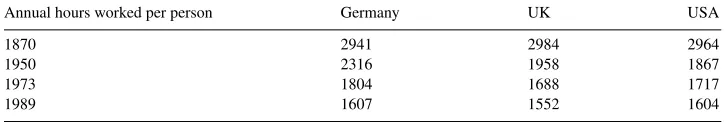
However, labor which still receives a large share of income in most countries, is sub-ject to important time-series and cross-section variations. Historically, Blanchard (1994) underlines that before the industrial revolution people enjoyed a relatively light work load in Europe, laboring only 100–150 days a year. This pattern was spatially and temporally widespread. With a reduction of population, and a resultant rise in wages in fifteenth-century England and the Netherlands, however, they worked only some 80–100 days. Later, with a higher population depressing wage rates, the peasants were forced to deploy their labor time in commercial and industrial pursuits, and accordingly had to work harder. Modern patterns of labor and leisure emerged only with the Industrial Revolution. The new norm was set around 300 days of 10 h a year. It continuously decreased since then. One should also mention that potential labor supply has sharply increased since 1750, as underlined by Fogel (1994). Consequently, the fraction of labor effectively supplied has strongly de-creased. Maddison (1991) provides data concerning labor supply in developed countries over the last century in Table 1.
More speculatively, one might be tempted to relate this steady decrease in labor supply over time as incomes grow in developed countries to the decline in their growth rate. Turning to cross-sections, the evidence is extremely scarce. For a sub-set of developing countries, Smith-Morris (1990) provides some comparative data that suggest a correlation between manufacturing weekly working hours and the growth rate during the 1980s. Asian coun-tries, where the working week was often above 50 h, enjoyed healthy growth rates during the period. By contrast, African countries, whose growth rates were often negative during the
pe-Table 1
The evolution of labor supply in developed economies
Annual hours worked per person Germany UK USA
1870 2941 2984 2964
1950 2316 1958 1867
1973 1804 1688 1717
riod, had a much shorter working week, around 40 h. How can this duality be explained? Do we need to invoke an exogenous parameter or is it the consequence of basic economic forces? Given their emphasis on technology, most endogenous growth models assume constant and exogenous labor supply and do not offer many insights to deal with this issue since causality runs only from labor supply to output and growth through the production func-tion.1 When endogenous labor supply is assumed in the growth literature, it is almost invariably under the hypothesis of a zero wage elasticity of leisure demand. Then, it is im-mediate that individual labor supply remains constant over time, as capital (or knowledge) is accumulated, which, as we have seen, is counter-factual. Only changes in the value of technological parameters or in preferences can lead to a change in the supply of labor. This assumption of zero income elasticity may be a good working assumption when studying issues such as the effects of taxation on economic activity when labor supply is only a channel of transmission as in the real-business cycle literature (see Kydland, 1995 for a review). The other defense of the zero wage elasticity of leisure demand is that balanced growth path can be obtained only under this assumption (Caballé and Santos, 1993).
However convenient it might be, this assumption is not sustainable in the long-run when the focus is on long-run growth. If labor supply is endogenous there is no a priori reason why theelasticity of labor supply with respect to the wage should precisely be zero. This zero elasticity is only a particular case in a general model. If anything goes, according to the empirical facts given by the survey of Pencavel (1986), the income elasticity of leisure demand is positive in the long-run and negative in the short-run in developed countries. The motivation of this paper is thus to explore “unbalanced” growth path where labor supply is allowed to vary over time as the time-series evolution in developed economies suggests.
We consider an overlapping-generations (OLG) model where labor is an essential input and where, depending on the amount of labor supplied, growth can be either positive or negative. Our reasons for choosing an OLG structure are the following. Since our goal is to study the global dynamic behavior of an economy under fairly general assumptions regarding labor supply, tractability constraints leave us either with Infinitely-Lived-Agents (ILA) and a simple dynastic utility function or with a simple OLG structure. The basic ILA framework does not receive much empirical support (Wilhelm, 1996) and, as remarked above, simple ILA structures with endogenous growth do not allow us to replicate some of the highlighted facts. By contrast, our OLG structure enables us to obtain results for more general paths than balanced growth paths using more general utility functions. Furthermore, our framework enables the derivation of some results for production functions that cannot be studied under the simple ILA approach.
Our results show that, when leisure and consumption are (gross) complements, we find asymptotically that endogenousgrowth does not occur, although it is both possible and socially desirable. Complementarity between leisure and consumption thus implies that people work too little and that “demand” limits to growth are met (in the sense of Kuznets, 1959). The increase in wealth induces a rise in wages. Due to the complementarity assump-tion, workers substitute part of their consumption for increased leisure. Working hours then
1There exists a sizable literature dealing with the endogenous evolution of fertility and its interactions with
decrease until production remains constant over time. A no-growth result is thus derived in an economy for which the assumptions were initially geared towards generating endoge-nous growth. As typical in an OLG structure, welfare is not maximized in the long-run since part of the work of the current generation benefits future generations (longer working hours today result in higher savings and consequently higher wages at the next period, but this is not internalized by the current generation in the absence of inter-generational altruism). In models with fixed labor supply, there is no possible Pareto improvement since a higher future consumption comes at the cost of a lower utility now. With variable labor supply, however, there is room for Pareto improvement. Increasing working hours can benefit all generations, including the first one. The disutility of a heavier work load can be compensated at the next period by higher returns to savings due to the harder work that will be performed by the next generation. This Pareto improvement also generates a positive growth rate. This cannot happen in a competitive equilibrium, because there is no enforceable contract that can link future generations with the current one. This result might support the view that labor supply should be constrained directly or indirectly through a tax mechanism, because people are not working hard enough. Such a rigidity of labor supply is crucial to maintain economic expansion over time. Our argument then goes against the traditional laisser-faire argument saying that labor supply should left unconstrained.
Under substitutability, which may constitute a good working assumption for low-income countries, multiple equilibria are possible. The model converges either towards a no-work poverty trap or towards a high-growth and heavy-work equilibrium. The intuition for the result is the following. In the high-growth case, as capital is accumulated, the successive generations experience an age of augmented expectations concerning the labor supply of the following generations. Then, the current generation works hard, since it expects that the next one to supply a higher quantity of labor and thus generate high yields for its savings. On the contrary, the poverty trap is entered after an age of diminished expectations concerning the labor supply of the following generations. Expectations of low yields induce a substitution of work for leisure, which has a negative effect on capital accumulation. The next generation then faces very low wages and low expectations, so that it effectively has even less incentive to supply labor heavily. Thus, the economy is stuck in a poverty trap. In our economy, people are not poor because they are lazy, rather they do not work because work does not pay. The popular causality is thus reversed. In such a poverty trap, only strong government intervention, sacrificing the welfare of the current generations, can set the economy on a positive growth path again.
The rest of the paper is organized as follows. Sections 2–4 explore, respectively, the case of zero, positive and negative income elasticity of leisure demand in a simple general equilibrium model with endogenous growth. Section 5 contains some final remarks.
2. Inelastic labor supply
the interest and the principal of their savings. They leave no bequest and we assume that the population of each generation remains constant, normalized to one. Labor supply is endogenous and maximum labor supply is equal to one. For simplicity we restrict our atten-tion to an environment, where the individual born intworks in periodtand consumes only in periodt+1. There is a disutility of work or, conversely, the representative individual is happier with increased leisure
Ut =U (lt, ct+1), Ul >0, Uc>0, Ull<0, Ucc<0, Ulc>0 (1)
withltbeing the individual leisure time(lt ≤1). There is only one good in this economy. It
can be used either as an investment or as a consumption good. The production function at the firm level is standard and assumes that labor is an essential input and it is homogenous of degree one in capital(kt)and labor
yt =Atktβ(1−lt)1−β. (2)
There is an externality at the aggregate level. Following Romer (1986), we suppose that the aggregate production function shows linear returns in the accumulated factor where upper-case letters denote economy-wide aggregates2
At =AK1t−β ⇒Yt =AKt(1−Lt)1−β. (3)
The economy is assumed to be perfectly competitive so thatwt =(1−β)AKt(1−Lt)−β
andrt =βA(1−Lt)1−β. Capital depreciates fully after one period. This impliesKt+1= wt(1−Lt).3 It is useful to define the zero-growth labor supply 1−L∗, which is such that Kt+1/Kt =1. After simplifications
L∗=1−((1−β)A)1/(β−1). (4) The individual budget constraint isct+1=wtrt+1(1−lt). Consequently, at the aggregate
level
Ct+1=Zt+1(1−Lt)1−β with Zt+1=β(1−β)A2Kt(1−Lt+1)1−β. (5)
The variableZt+1 can be viewed as an intertemporal total factor productivity parameter
for the generation born int. This variable, which pays a key role in the analysis below, is a function of the period total factor productivity parameterA, of the shares given to the factors
βand 1−β, the quantity of accumulated capital,Kt, and of labor supply int+1,Lt+1.
Young individuals born intmaximize their utility given the values of the different param-eters and variables in periodtand the rationally expected values of the parameters and vari-ables in periodt+1. Namely, if we assume the stability of the production function and tastes, individuals optimize overltgivenLt, Kt andLt+1. The consumer program can be written
Maxlt U (lt, ct+1),
subject to : (1−lt)wtrt+1=ct+1. (6)
2As usual, the accumulated factor is capital in its broadest sense, be it knowledge, human or physical capital. A
more complete discussion on this issue is provided further in this paper.
3Our results are robust to less extreme assumptions concerning depreciation. They hold as long as the depreciation
From (5) and (6), a simple demand functionl(Zt+1)for aggregate leisure can be defined.
A temporary equilibrium in periodtis defined by the maximization above and the clearing of all markets. The reduced form of the model is thus given by
(l(Z
t+1)−Lt =0 with Zt+1=β(1−β)A2Kt(1−Lt+1)1−β, Kt+1=(1−β)AKt(1−Lt)1−β.
(7)
In this section, we assume that the income elasticity of leisure demand is zero
(a0) Inelasticity of leisure demand : ∂lt(Zt)
∂Zt+1
=0 ∀Zt+1.
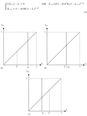
Under assumption (a0), the solution to (5) is such that the income effect exactly offsets the substitution effect, which implies that the choice of the effort is constant and independent of the expected returns of the savings. The dynamic behavior of the capital stock is then given byKt+1/Kt =(1−β)A(1−L)1−β. Consider for instanceU=ln(lt)+αln(ct+1).
One findslt =Lt =1/(1+α)andKt+1/Kt =(1−β)A(α/(1+α))1−β. Thus, depending
on the value ofα, the economy experiences steady negative growth (lowα), a no-growth steady-state or steady positive growth (highα). See Fig. 1 for an illustration.
As a conclusion for this section, note that the inelasticity-of-labor-supply assumption is very convenient because it amounts to neglecting future events and thus implies a constant demand for leisure. However, this simplification is obtained with an important loss of generality. Nonetheless, except for Eriksson (1996) in a continuous time framework (but in his case labor supply does not affect accumulation) or Hahn (1989) for neoclassical growth models, papers dealing with growth and endogenous labor supply usually adopt this assumption. The fact is that labor supply in these papers is just an ingredient not their specific object of study, which is either the endogenous fluctuations of the economy or the impact of taxation (see Benhabib and Perli, 1994; Jones et al., 1993 or King et al., 1988 for examples of such treatments). The rest of the paper explores the behavior of our prototype endogenous growth model with endogenous labor supply when the assumption of zero wage elasticity is relaxed.
3. Substitutability between leisure and consumption
A first justification for this section is that substitutability between leisure and consumption should be considered as a theoretical possibility. It is also empirically relevant for low levels of income as assumed by traditional labor supply curves. Assume the following:
(a1) Continuity:l(Zt+1)is continuous and twice differentiable.
(a2) Substitutability:∂l(Zt+1)/∂Zt+1<0.
(a3) Convexity:∂2l(Zt+1)/∂Zt2+1>0.
(a4) Boundary conditions: limZt+1→0l(Zt+1)=1 and limZt+1→∞l(Zt+1)=0.
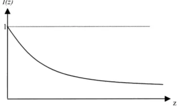
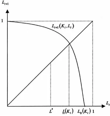
Assumption (a1) requires that the demand for leisure is well defined. Assumption (a2) is the main assumption of substitutability between leisure and consumption. Assumption (a3) ensures that the labor supply curve must be concave (or convex demand for leisure). Note that the boundary conditions in (a4) could be relaxed. We just need labor supply to be able to create positive and negative growth. The use of 0 and 1 will just make the proofs easier. These assumptions are summarized on Fig. 2. They lead to the following lemma.
Lemma 1. Assumptions(a1)–(a4)define a mapLt+1(Lt, Kt)with the following properties:
Fig. 2. The leisure demand function under substitutability.
(P2) ∂2Lt+1(Lt, Kt)/∂L2t ≤0.
(P3) For anyKt >0,Lt+1(1, Kt)=1and∂Lt+1(Lt, Kt)/∂Lt|Lt=1=0.
(P4) limLt→0Lt+1(Lt, Kt)= −∞and∀ε∈(0,1),∃Kt such asLt+1(ε, Kt)=0.
Proof. From Eq. (7), we obtain directlyl(Zt+1)−Lt =0 withZt+1=β(1−β)A2Kt(1− Lt+1)1−β. A direct application of the implicit function theorem yields ∂Lt+1/∂Kt = −(∂Zt+1/∂Kt)/(∂Zt+1/∂Lt+1) ≥ 0. Another application of the same theorem implies ∂Lt+1/∂Lt =(∂l(Zt+1)/∂Zt+1(∂Zt+1/∂Lt+1))−1 ≥0, which ends the proof of (P1). A
further application of the same theorem yields (P2). Note that ifLt =1, thenKt+1 =0
which impliesKt+2 = 0 and thusZt+2+0. Due to the disutility of labor, this implies Lt+1=1. Since∂Lt/∂Lt+1= −β(1−β)2A2Kt(1−Lt+1)−β∂l(Zt+1)/∂Zt+1and since Lt =1 impliesLt+1=1 then∂Lt+1(Lt, Kt)/∂Lt|Lt=1=0. This proves (P3). By (a2) and
(a4),Ltcan be zero only whenZt+1is infinite. This is the case for anyKt >0 only when Lt+1is negative and infinite. By (a2) and (a4), for anyεbetween 0 and 1 there is a value of Zt+1such thatLt(Zt+1(ε))=ε. Note then thatKt =Zt+1(ε)/β(1−β)A2corresponds
toLt+1=0, which proves (P4).
SinceLt+1is monotonically increasing inLtand can take negative values and any positive
values below 1, for anyKt, there is a unique the fixed pointL(Kt)ofLt+1(Lt, Kt)such
thatL(Kt)=Lt+1(L(Kt), Kt)(andLt 6=1). This (temporary) fixed point is the demand
for leisure int such that the same demand is expected int +1. Define also the (unique) demand for leisure intif zero leisure demand is expected int+1,L0(Kt), which is such
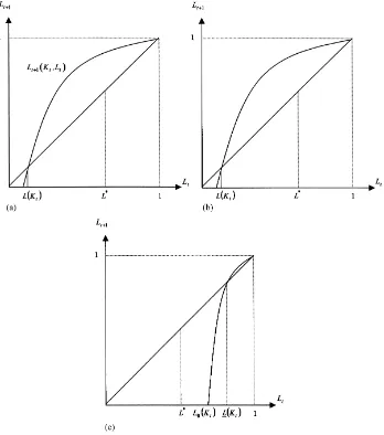
thatLt+1(L0(Kt), Kt)=0. Fig. 3 gives a simple diagrammatic illustration of some typical
situations. For example the CES utility functionUt =lt1−σ/(1−σ )+γ ct1+−1σ/(1−σ )with γ >0 and 0< σ <1 satisfies assumptions (a1)–(a4) (and consequently (P1)–(P4)).
Note that this forward-looking dynamic system is strongly non-linear. Hence, there is no hope of generating a complete analytical solution of our problem. Nonetheless, some results can be derived.
Result 1. Under(a1)–(a4),there exist two no-growth steady-states.
Proof. If the economy expectsLt+1=1, (P3) impliesLt =1. Then,Kt+1 =0 and the
Fig. 3. Substitutability between leisure and consumption: (a) a typical case; (b) growth; (c) inevitable recession.
the trivial steady-state. We can also defineK∗such thatLt+1(L∗, K∗) = L∗. The
exis-tence and uniqueness ofK∗directly stem from the intermediate value theorem with (a1),
(a2) and (a4). We can check easily that(L∗, K∗)is a no-growth steady-state with strictly positive output since (i) Kt+1(L∗, K∗) = K∗ and (ii) demanding L∗ is self-fulfilling.
From Eq. (4), no other level of leisure demand except for unity can imply a steady-state. Any level of capital, except for K∗, makes the demand L∗ inconsistent with rational
Result 2. Under(a1)–(a4),there exists at least one equilibrium path with sustained positive growth for a large enough initial K. It is such that the demand for leisure tends to zero asymptotically.
Proof. Proof in Appendix A.
The argument runs as follows. IfLt ≥ L(Kt), this implies for somet′ > t,Lt′ > L∗
and thus negative growth untilK < K∗. There is also a neighborhood left ofL(Kt), for
which the demand for leisure ends up being superior toL∗. This implies the same outcome as previously. Note also thatLt < L0(Kt)impliesLt+1<0, which is inconsistent. There
is also a neighborhood right ofL0(Kt)such that for somet′> t,Lt′ < L0(Kt′)and thus
Lt′+1<0 which is again inconsistent. Since no point can belong to both neighborhoods,
there is at least one equilibrium path with sustained growth betweenL0andL. Moreover,
sinceLt < L0(Kt),Lis driven to zero whenKbecomes very large. Any equilibrium with
growth then implies that leisure time should converge to zero.
Result 3. Under(a1)–(a4),the equilibrium path with growth is unique.
Proof. From Lemma 1, considerLt+2(Lt+1(Lt, Kt), Kt+1(Lt, Kt)). Full differentiation
leads to dLt+2/dLt =∂Lt+2/∂Lt+1×∂Lt+1/∂Lt+∂Lt+2/∂Kt+1×∂Kt+1/∂Lt. Since ∂Lτ+1/∂Lτ ≥0, then dLt+2/dLt ≥∂Lt+2/∂Kt+1×∂Kt+1/∂Lt. After replacement, this
implies dLt+2/dLt ≥(1−Lt+2)/(1−β)×Kt+1/Kt >0. Note further that forKlarge
enough,Lt < βandKt+1/Kt >1. This implies dLt+2/dLt >1. Thus, if for any level
of capital, two different levels of leisure demand were in equilibrium, the two equilibrium paths would be diverging. This is impossible sinceLtends towards 0. Hence, the growth
path is unique.
Result 4. Under(a1)–(a4),there exists at least one equilibrium path with negative growth. Negative growth is the only outcome whenKis less thanK∗.
Proof. The first part of the result is straightforward: the trivial steady-state is always possible (see the proof of Result 1). Sustained positive growth requiresLt < L∗for anytand{Lt}
decreasing. Then, if we reverse the time scale{L−t}is increasing and bounded from above.
Then it must converge toward a level lower thanL∗(if it was converging towardsL > L∗, then growth would be impossible in the first stages). From Result 3, the lowest level of capital consistent with that assertion (i.e.,L(Kt)=L∗) isK∗. By contraposition,K < K∗
implies negative growth.
Corollary 1. The non-trivial steady-state with no growth is unstable.
Proof. This corollary stems directly from Results 1 and 4.
steady-state is eventually reached. Even above the threshold, the trivial steady-state cannot be ruled out. The trivial steady-state can be interpreted as a poverty trap.4
The only equilibrium path that involves sustained growth also implies a sustained decrease of leisure demand towards zero. The intuition of the result is the following. The current generation works hard because it expects the next generation to work very hard as well and, in so doing, to offer the future retired people high yields for their savings. The next generation has the same beliefs. Since, the amount of accumulated capital is higher, wages are higher. The incentive to substitute leisure for work is even stronger. Thus, labor supply has to increase over time and it tends to unity.5
By contrast, when individuals expect low returns for their savings, their demand for leisure is high, so that capital at the next period is scarce and wages are low. This makes work even less attractive for the next generation, which confirms previous expectations. Labor supply decreases until the trivial steady-state is reached.6 This coordination failure arises because of the OLG structure where no contract between generations (all committing to a high supply of labor) is feasible. The externality in the aggregate production function (which enables growth) is usually at the root of the inefficiencies in endogenous growth models. Here, it only plays a very minor role. Even if savers were to receive the full marginal product of their investments, it would only affectZt+1multiplicatively by a factor 1/(1−β).
This would modifyK∗but would leave Results 1–4 unchanged.
When the economy is in the low equilibrium, there is no possibility to escape it in under laisser-faire. This argument may act as a rationale for government intervention (justified only by a Utilitarian and not a Pareto criterion) in low income countries, for which the substitutability assumption might be valid. This intervention may not create too many dis-tortions, since it suffices for the government to intervene for a finite number of periods. Once the high growth equilibrium path is triggered, no more intervention is required.
Results 1–4 hold under well-behaved utility functions exhibiting substitutability between leisure and consumption.7 If individuals consume when young as well as when old, results get more complicated. However, it seems natural to focus on the assumption of
comple-4When the depreciation rate is strictly below 1 or when minimum labor supply is restricted to be strictly positive,
the low steady-state implies a strictly positive level of capital. Note also that this poverty trap does not stem from restrictions on the production function as in Azariadis and Drazen (1990) (i.e., an exogenous non-convexity in the returns of the production function.) but it results from the structure of tastes, initial conditions and expectations. Of course, the model can also be “growth-constrained” if the minimum labor supply is high enough to generate growth whatever the expectations or if the depreciation rate is zero.
5Note that upper-corner solutions for labor supply are impossible because of the infinite marginal utility of
leisure (as assumed implicitly with the demand function), when leisure demand is close to zero.
6An interpretation in terms of product multiplicity can be also developed (withlfiguring some index of
con-sumption of goods produced with constant returns such as agricultural products or manufactured goods produced with a traditional technology.
7They are also robust to the formation of expectations. The rational expectation assumption might look at bit
strong. If one thinks of simple possible rules of thumb, one may supplyLtsuch thatLt+1=Ltwhere one is unable to forecast the changes of economic conditions due to the accumulation of capital. Under this rule of thumb, we can see thatLt=L(Kt). Then, we have three different possible situations. IfK=K∗, then the economy stays at the (unstable) steady-state. IfK > K∗, thenL
t> L∗. The economy keeps growing:Kt+1< KtandLt+1< Lt. Captial grows unbounded, whereas leisure tends to zero. IfK < K∗, thenL
mentarity or multiplicative separability of the two consumptions. As a consequence, in-tertemporal consumption smoothing leads to both consumption levels to be “tied” in the sense that pessimistic expectations about future returns do not induce people to substitute future consumption for present consumption but consumption for leisure. The essence of the results then should not be modified by this refinement of the model.
Finally, note that sociological theories of growth often emphasize the importance of culture in the process of development. Cultural values are supposed to govern the attitude towards work. Here, we simply assume, that the economic returns are higher when one works more. If we accept here the idea that consumption and leisure are substitutes when people are poor, there exist multiple equilibria. Consequently, poverty may not be the result of cultural values through a direct causality, but a matter of self-fulfilling expectations and initial conditions. Nonetheless, sociological explanations may still have a part to play since expectations matter. Furthermore, to escape the trivial (or low) steady-state, Weber (1930) emphasizes some form of irrationality with respect to our specification for utility. In his introduction, he underlines that (With Protestantism)man is dominated by the making of money, by acquisition as the ultimate purpose of his life. [. . .]Economic acquisition is no longer subordinated to man as the means for the satisfaction of material needs.
4. Complementarity between leisure and consumption
The case for which leisure and consumption are substitutes is empirically weakly relevant for developed economies, since most studies surveyed by Pencavel (1986) show a long-run complementarity between those two goods. Another reason to justify this complementar-ity assumption is thattime is the ultimate scarce resource as consumption goods become abundant. Even with a longer life-expectancy, our lifetimes still remain bounded, whereas there is no reason for consumption to be bounded in the future. This view states that time is valued for its own sake. Becker (1965) takes a more materialistic approach (where time has no value as such) and underlines that utility is derived from both the amount of con-sumption and the time devoted to concon-sumption with a complementarity between the two. Both approaches are equivalent in our model. Assume the following:
(a5) Continuity:l(Zt+1)is continuous and differentiable.
(a6) Complementarity:∂l(Zt+1)/∂Zt+1>0.
(a7) Boundary conditions: limZt+1→+∞l(Zt+1)∈(L
∗,1)and lim
Zt+1→0l(Zt+1) < L
∗.
Assumption (a5) ensures that the demand function is well-defined. Assumption (a6) states the complementarity between consumption and leisure. Assumption (a7) is just here to ensure that leisure demand can be low enough to imply positive growth or high enough to yield negative growth. These assumptions, which are summarized on Fig. 4, lead to the following lemma.
Lemma 2. Assumptions(a5)–(a7)define a mapLt+1(Lt, Kt)with the following properties:
(P5)∂Lt+1(Lt, Kt)/∂Kt ≥0and∂Lt+1(Lt, Kt)/∂Lt ≤0.
Fig. 4. The leisure demand function under complementarity.
Proof. From (7) and as in Lemma 1, the implicit function theorem yields∂Lt+1/∂Kt = (∂Zt+1/∂Kt)/(∂Zt+1/∂Lt+1)≥0 and∂Lt+1/∂Lt =(∂l(Zt+1)/∂Zt+1(∂Zt+1/∂Lt+1))−1.
Eqs. (7) and (a6) show that this last term is negative. This demonstrates (P5). From the monotonicity ofLt+1(Lt, Kt)and (a7), the lower limit ofLis reached only whenZtends
to zero. When Kt > 0, this can be achieved only forLt+1 = 0. Similarly, the upper
limit ofLis reached only whenZ tends to infinity, which requires,Lt+1 = −∞. This
proves (P6).
These properties ensure the existence of the (temporary) fixed-pointL(Kt)and ofL0(Kt).
They are such thatL(Kt)≤ L0(Kt)(refer to Fig. 5 for a diagrammatic exposition). For
example the CES utility functionUt =lt1−σ/(1−σ )+γ ct1+−1σ/(1−σ )withγ >0 and σ >1 satisfies assumptions (a5)–(a7). Our basic result for this section is then quite easy to establish.
Result 5. Under(a5)–(a7),sustained positive and sustained negative growth are impossi-ble.
Proof. The proof is by contradiction. Sustained positive growth requiresL < L∗for capital to keep growing. This leadsKto become superior toK∗and thusLt+1(Lt, Kt)to become
such thatL(K)andL0(K)are superior toL∗. For capital to continue to grow, we still need Lt < L∗. This implies thatLt+1> L∗is expected. Then, when these rational expectations
are fulfilled, it meansKt+2 < Kt+1. Thus, sustained positive growth is impossible and
the same argument runs with negative growth. The economy cannot experience explosive cycles either, since the growth rate is bounded by(1−β)A.
The corollary of this result is that the economy in the long-run is either at the steady-state
(L∗, K∗)or experiencing small scale fluctuations around the steady-state.8 In other words, the Romer assumption coupled with a positive income elasticity of leisure demand implies a Solow-type outcome. The intuition is that, when wealth increases, individuals tend to work less due to an increased demand for leisure. Working hours then decrease, until production remains constant over time. Unsurprisingly, depending on the slope ofLt+1(Lt, Kt)at (L∗, K∗), the steady-state is either locally stable (if the slope is superior to−1) or unstable.9 Moreover, our results can be extended to another class of production functions, which can be studied only in an OLG framework.
Result 6. Sustained positive or negative growth is impossible with the production function
yt =AK1t−β+µk β
t (1−lt)1−β and withUt =lt1−σ/(1−σ )+γ ct1+−1σ/(1−σ )(γ >0and σ >1).
Proof. Proof in Appendix B.
With constant labor supply, this production function should yield explosive rates of growth. Result 6 shows that the no-growth result can be extended for such a production function when utility is CES.
A possible objection to these two results could be raised using the fact that our engine of growth is very specific. In particular, do our results hold with what is usually referred to in endogenous growth models as “accumulation of knowledge” or “technological progress” (Romer, 1990 and many subsequent papers)? These more sophisticated models of endoge-nous growth use a constant returns to scale production function for the consumption good, along with another sector (R& D) for which the creation of new knowledge is a linear function of existing knowledge and an increasing function of labor employed in this sector. Technically, both frameworks are the same, yielding the same kind of results (see Gross-man and HelpGross-man, 1994). The only differences rest with the treatment of the competitive assumption. Our conjecture is that in such models, growth would imply a decrease of the
8As in the previous section, this result is robust to the formation of expectations. If one expectsL
t+1 =Lt, whenKt> K∗, one getsLt+1> L∗and hence negative growth. WhenKt< K∗, one getsLt+1< L∗and hence
positive growth.
9See Cazzavillan et al. (1998) for a detailed analysis of fluctuations in a model with less than linear returns to
labor supplied in the R& D sector (growth should reduce the incentive to supply labor in the manufacturing sector, which in turn reduces the value of patents). Thus, the same type of mechanism would drive sustained growth to an end. If instead of knowledge, human capital was accumulated the results should also remain valid as long as the demand for leisure increases in the income.
This stagnation result would not be very worrying if this situation was Pareto-optimal (and it would be so in an ILA framework with a CES utility function after correcting for the externality in the production function). However, this is not the case here.
Result 7. When the economy is at its steady-state, it is possible to improve the welfare of all future generations including the current one by setting labor supply exogenously. This welfare improvement implies positive growth.
Proof. See Appendix C for a formal proof.
Then, although endogenous growth is possible and socially profitable, it does not take place. A Pareto-improvement is possible because a small increase in the labor supply of the future generations (i.e., higher consumption) compensates for a small increase in the labor supply of the current generation. In contrast to many endogenous growth models, the inefficiency does not come from insufficient investment in R& D or in physical capital, but from sub-optimal labor supply. Typically, in models with exogenous labor supply, the unregulated growth rate is equal to the optimal growth rate minus a constant, which depends on the difference between private and social returns. In this model, even when this wedge is filled, our complementarity between consumption and labor still drives the growth process to a complete standstill. Indeed, a subsidy on savings (a standard recommendation of en-dogenous growth models) raises the intertemporal returns to labor, which depresses labor supply even more. To restore efficiency, it may be possible to tax investment or savings in order to induce workers to work more (instead of subsidizing it in models with constrained labor supply). It may also be possible to directly compel people to work sufficiently so that perpetual growth should occur. This may be very hard to implement since it is possible to extend the model realistically with every generation voting on taxes or working hours. This voting process should bring us back to Result 5.
5. Concluding remarks
This assumption, however, does make sense empirically. We face here an apparent con-tradiction. Although the model predicts that growth should stop, it still occurs. It might simply be that we are converging to a steady-state we have not reached yet, but that even-tually demand limits to growth will appear. Yet, many other candidate explanations can be at work to explain theex-postrigidity of labor supply, but most of them must be ruled out regarding our case. Traditional labor economics stresses the importance of labor external-ities, indivisibilities and increasing returns to labor effectively supplied. But except from extreme forms of indivisibilities (individual returns are zero if one works less than 1−L∗), this may not be sufficient to reverse Results 4 and 5.
One possible way to explain the persistence of high labor supply is the existence of some “oligarchic wealth”. Typically the only engine of growth usually found in economic models is the willingness to consume more. Given this objective, people work, accumulate, learn or trade indefinitely to maximize their intertemporal utility assuming. When wealth is “democratic” (i.e., all goods can be multiplied and produced in ever increasing quantities), the model shows that demand limits to growth should be reached. By contrast, one may assume that total social reward within a group is fixed (i.e., there can be only one winner) or that honors and positions are sought for their own sake (more generally, there are goods in limited supply whatever the state of development). Then unlike the quest for consump-tion, the quest for social reward (for instance being the richest man in the village, the most quoted economist, or owning a painting by Vermeer) is endless since aggregate satiation is impossible.
Cole et al. (1992) proposed a matching model where people are interested in physical attributes and thus have an incentive to work in order to be able to mate with the best partners. In other papers, Corneo and Jeanne (1999) or Fershtman et al. (1996) introduced directly a concern for social status in the utility function. This type of argument is consistent with a deeper observation of the empirical data provided by Pencavel (1986). The average working time may be declining, but many highly qualified and wealthy people still work 60 h a week, very often at a high cost for their family or their health. The elite may be part of a “rat race” from which growth might be only a side-effect.
As a final point, this paper has explored the behavior of a standard growth model with endogenous labor supply. We showed that with a negative income elasticity of labor supply, the economy converges either towards a level equilibrium or towards a high growth and high labor supply situation, thus replicating the situation in many developing countries. By contrast, when consumption and leisure are complement, demand for leisure should increase as the economy grows richer until a no-growth steady-state is reached. Further work should focus on the generality of this result. Moreover, new arguments able to re-store the possibility of positive growth should enrich our understanding of the growth process.
Acknowledgements
Financial support from the French Ministry for Research and Technology is also gratefully K∗, capital eventually falls belowK∗, which is in contradiction with sustained positive growth.
The second step is to show that there is a neighborhood left ofL(K)such that sustained growth is impossible for anyLin this neighborhood. For sustained positive growth,Kt+1> Kt is required. Note thatL(Kt+1) < Lt+1(Lt, Kt)=L(Kt), sinceL(K)is decreasing in Kdue to (P1). By continuity, there is a neighborhoodI1(K), left ofL(K)such that for all x ∈I1(K), we haveL(Kt+1(x)) < Lt+1(x, Kt)≤x ≤L(K). WhenLt+1> L(Kt), this
impliesLt+2> Lt+1and a continuous decline of labor supply until capital eventually falls
belowK∗. Recursively, we haveI2(K), left ofI1(K)and such thatLt+2(Lt+1, Kt+1) <
Thus, to get sustained growth, we needLt be left ofI (Kt). Otherwise, expectations would
be dynamically inconsistent with the growth hypothesis (Kwould end up being superior to
K∗, see step 1). Note thatLt < L(Kt), a necessary condition for positive sustained growth,
implies that leisure demand must tend to zero.
For the third step, note that demandingLt =L0(Kt)impliesLt+1 =0 andLt+2<0,
which is inconsistent with rational expectations. By continuity, there is a neighborhood
J1(K), right of L0(K) such that it would be dynamically inconsistent to demandLt ∈ J1(K). In fact, demandingLt impliesLt+1< L0(Kt+1)which leads to inconsistencies in
Thus for sustained growth, a necessary condition is that anyLmust be left ofI (K)and right ofJ (K). If leisure demand is on the right ofI (K), the path of labor supply is not decreasing enough (leading eventually capital to fall belowK∗), whereas if it is on the left ofJ (K), it is decreasing too fast to be dynamically consistent. A growth path will exist if, for anyK > K∗, there is at least one sequence of leisure demand not inconsistent with rational expectations. In particular, if there is anyLtleft ofI (Kt)and right ofJ (Kt), thenLt+nis left ofI (Kt+1)
always consistent with rational expectations for all future periods). This is sufficient for growth to occur since:Lt < L∗ ⇒Kt+1 > Kt. Note that capital must be initially large
enough forL0(K) < L∗.
For the fourth step, it remains to show that, no point can belong to both neighborhoods,
I (K)andJ (K). Suppose there isLt ∈I (K)∩J (K), then there must beτ ≥tsuch that Lτ+1> Lτ andLτ+1< L0(Kτ+1). These last two conditions implyL0(Kτ+1) > Lτ. By
definition, we also haveL0(Kτ) > L0(Kτ+1). Then, we must observeLτ > L0(Kτ). This
leads to a contradiction since we needLτ < L0(Kτ), otherwise it would meanLτ+1 =
0. Hence, there always exists at least one equilibrium path involving positive sustained growth.
Appendix B. Proof of Result 6
SinceUt =lt1−σ/(1−σ )+γ c1t+−1σ/(1−σ )(withγ >0 andσ >1) andYt =AK1t+µ(1− Lt)1−β, the labor supply that leaves initial conditions constant is no longer independent of K. DefineL∗(Kt)such thatKt+1/Kt = 1, i.e.,(1−β)AKµt(1−L∗(Kt))1−β = 1. In
order for sustained positive growth to be possible, we needLt < L∗(Kt)under the rational
expectationLt+1< L∗(Kt+1). Individual maximization implies
The temporary equilibrium is then such thatlt =Lt, so we find
Appendix C. Proof of Result 7
In the steady-state(L∗, K∗), the utility of each generation is
U∗=U (L∗, (1−β)AK∗(1−L∗)1−β) with L∗=1−((1−β)A)−1/(1−β). (C.1) andL∗satisfies
dU (l, (1−β)βA2(1−L∗)−β(1−l)K∗(1−L∗)1−β)
dl =0, (C.2)
Ul(L∗, (1−β)AK∗(1−L∗)1−β)
−(1−β)βA2K∗(1−L∗)1−2βUc(L∗, (1−β)AK∗(1−L∗)1−β)=0. (C.3)
The authority can fixL∗∗forever. If all excess production for(1−L∗∗) > (1−L∗)is given to the young generation, we observe then
1U=1L×Ul(L∗∗, (1−β)AK∗(1−L∗∗)1−β)
−1C×Uc(L∗∗, (1−β)AK∗(1−L∗∗)1−β). (C.4)
ForL∗∗=L∗, it implies
1U
1L =Ul(L
∗, (1−β)
AK∗(1−L∗)1−β)
−(1−β)A2K∗(1−L∗)1−2βUc(L∗, (1−β)AK∗(1−L∗)1−β). (C.5)
In this case, using (C.3), one can check that the RHS of this expression is strictly positive. Consequently, by continuity there existsL∗∗ < L∗such that we can setL =L∗∗. In that case, the generation born int−1 receives the same income, whereas the generation born in
tis better-off. All the generations born aftertare also better off since they work the same and consume more than the generation born int.
References
Azariadis, C., Drazen, A., 1990. Threshold externalities in economic development. Quarterly Journal of Economics 105, 501–526.
Becker, G., 1965. A theory of the allocation of time. Economic Journal 75, 493–517.
Becker, G., Murphy, K., Tamura, R., 1990. Human capital fertility and economic growth. Journal of Political Economy 98, S12–S37.
Benhabib, J., Perli, R., 1994. Uniqueness and indeterminacy: on the dynamics of endogenous growth. Journal of Economic Theory 63, 113–142.
Blanchard, I. (Ed), 1994. Labour and Leisure in Historical Perspective: Thirteenth to Twentieth Centuries. Franz Steiner, Stuttgart.
Caballé, J., Santos, M., 1993. On endogenous growth with physical and human capital. Journal of Political Economy 101, 1042–1068.
Cole, H., Mailath, G., Postlewaite, A., 1992. Social norms, savings behavior, and growth. Journal of Political Economy 100, 1126–1152.
Corneo, G., Jeanne, O., 1999. Pecuniary emulation inequality and growth. European Economic Review 43, 1665–1678.
Eriksson, K., 1996, Economic growth with endogenous labor supply. European Journal of Political Economy 12, 533-544.
Fershtman, C., Murphy, K., Weiss, Y., 1996. Social status education and growth. Journal of Political Economy 104, 108–132.
Fogel, R., 1994. Economic growth, population theory, and physiology: the bearing of long-term processes on the making of economic policy. American Economic Review 84, 369–395.
Grossman, G., Helpman, E., 1994. Technology and growth. National Bureau of Economic Research Working Paper 4926.
Hahn, F., 1989. Solovian models of growth. University of Cambridge Economic Theory Discussion Paper 137. Jones, L., Manuelli, R., Rossi, P., 1993. Optimal taxation in models of endogenous growth. Journal of Political
Economy 101, 485–517.
King, R., Plosser, C., Rebelo, S., 1988 . Production growth and business cycles. I. The basic neo-classical model. Journal of Monetary Economics 21, 195–232.
Kuznets, S., 1959. Six Lectures on Economic Growth. Free Press, New York.
Kydland, F., 1995, Business cycles and aggregate labor market fluctuations. In: Cooley, T. (Ed.), Frontiers of Business Cycle Research. Princeton University Press, Princeton, NJ.
Maddison, A., 1991. Dynamic Forces in Capitalist Development. Oxford University Press, Oxford.
Pencavel, J., 1986. Labor supply of men. In: Ashenfelter, O, Layard, R. (Eds.), Handbook of Labor Economics, Vol. I. North-Holland, Amsterdam, pp. 1–103.
Romer, P., 1986. Increasing returns and long-run growth. Journal of Political Economy 94, 1002–1037. Romer, P., 1990. Endogenous technical change. Journal of Political Economy 98, S71–S102.
Smith-Morris, M. (Ed.), 1990. The Economist Book of Vital World Statistics. The Economist Books, London. Weber, M., 1930. The Protestant Ethic and the Spirit of Capitalism. Unwin, London.