*Corresponding author: Tel.: #1-817-921-7194/7527; fax: #1-814-921-7227.
E-mail address:[email protected] (R.V. Ramasesh).
Lot streaming in multistage production systems
Ranga V. Ramasesh!,
*, Haizhen Fu", Duncan K.H. Fong#, Jack C. Hayya#
!M.J. Neeley School of Business, Texas Christian University, Fort Worth, TX 76129, USA "I2 Technologies, Irving, TX 75039, USA
#Pennsylvania State University, University Park, PA 16802, USA
Received 5 February 1999; accepted 5 October 1999
Abstract
Lot streaming is a procedure in which a production lot is split into smaller sub-lots and moved to the next processing stage so that operations at successive stages of a multistage manufacturing system can be overlapped in time. Lot streaming reduces the manufacturing lead time and thereby provides an opportunity to lower the costs of holding work-in-process inventories. In this paper, we present an economic production lot size model that minimizes the total relevant cost when lot streaming is used. Using illustrative numerical examples, we show that our model can yield signi"cant cost economies compared to the traditional approaches. ( 2000 Elsevier Science B.V. All rights reserved.
Keywords: Lot streaming; Economic lot sizing; Multistage production systems
1. Introduction
Lot streaming is an appealing concept in produc-tion management with almost universal applicaproduc-tion in multistage manufacturing systems. Lot stream-ing is a procedure in which a large production lot is split into smaller sub-lots and the operations at the successive stages are overlapped in time. The sub-lots are transported from one stage to the next for processing without waiting for the entire produc-tion lot to be processed at the earlier stage before being moved to the next stage. A major bene"t of lot streaming is the reduction in the manufacturing cycle time for an item, which requires several opera-tions to be performed in a speci"c order. As an
illustration of this bene"t, suppose the lot size of a certain item is 100 units and its production involves operations on three machines. Let the pro-cessing times be 2, 3, and 4 minutes per unit, and the setup times 50, 75, and 75 minutes on the three machines. Assuming no scheduling delays and transportation times, the production lot of 100 units will be completed in 1100 minutes. However, if we split the production lot into two sub-lots of 50 units each and move a sub-lot as soon as it is"nished to the next stage for processing, then the processing of the two lots will be completed in 850 minutes. Thus, in this example, lot streaming has reduced the manu-facturing lead-time by about 23%. This results in savings in cost due to reduction in work-in-process (WIP) inventories, reduction in#oor space require-ments, and smaller material handling equipment. If these savings outweigh the incremental transporta-tion costs that may be incurred due to the move-ment of several smaller sub-lots rather than just
one complete lot, overall cost economies are achieved.
In this paper, we focus on the problem of deter-mining the optimal lot size for a single item in a multistage manufacturing system when a lot-streaming procedure is adopted and the costs asso-ciated with WIP inventories are taken into account. We derive the total cost function and develop a solution procedure to determine the optimal lot size to minimize the total relevant cost. We develop an economic production lot-sizing model that deals with re"nements to the models currently in the literature and we endeavor to make two speci"c contributions. First, we present a more realistic model that explicitly recognizes the setup time for each operation, transportation time for each sub-lot from one operation to another, and the planned scheduling delays or the waiting times at each op-eration. Second, we extend the application of the lot streaming procedure to multistage systems thus going beyond the currently available models of only two-stage systems. Our model yields an opti-mal lot size that results in a lower total cost compared to the traditional approaches in which (a) the lot size is determined based only on the"nal or "nished product stage of a multistage produc-tion system, and (b) the lot streaming procedure is not used. Using illustrative numerical examples, we show that our model yields signi"cant savings in total costs compared to the traditional approaches and then discuss its implications for managerial decision making.
Our paper is organized as follows: In Section 2, we review the relevant literature and outline the speci"c extensions this paper endeavors to make. In Section 3, we state the assumptions underlying our model, and the notations used in its development. In Section 4, we derive the expressions for the manufacturing cycle time and the WIP inventory as functions of the production lot size and the number of sub-lots. In Section 5, we"rst develop a general expression of the total relevant cost (the sum of the setup cost, the transport cost, and the holding costs of both the WIP and the "nished product inven-tory) as a function of the lot size and the sub-lot size. We then analyze two cases: (1) a special case in which the production rates at all stages of manufac-turing are identical and (2) a more general case in
which the production rates at all stages need not be identical but the number of sub-lots is pre-speci"ed. We use numerical examples to compare the total cost performance of our approach with that of the classical lot-sizing approach in which lot streaming is not employed and the lot size is determined based only on the"nishing stage. Finally, in Section 6, we provide a summary stating our conclusions and their implications for managerial decision making.
2. Overview of the relevant literature
The literature on inventory modeling is extensive and several studies have explored the concepts re-lated to the recognition of WIP inventories, lot splitting, and overlapping of operations in multi-stage manufacturing systems, under several di! er-ent assumptions and in di!erent contexts. In this section, our goal is not to present an extensive review of the literature but to provide an overview of a small and representative sample of related studies to facilitate the positioning of our paper appropriately. In doing this, we "nd it useful to recognize two main streams of studies, one dealing with the scheduling decisions and the other addressing the lot sizing decisions. The scheduling studies have been concerned with the shop perfor-mance measures such as the mean#ow time and the variability of #ow times. On the other hand, lot sizing studies have been concerned with the e!ect of the reduction in the total manufacturing cycle time on the costs of holding WIP inventory in relation to additional transportation costs. Due to the com-plexity of the multistage production}inventory systems and the many factors in#uencing the prob-lem, analytical studies in general have developed models addressing the scheduling and the lot sizing decisionsindependentlyalthough the two decisions are intricately connected in practical settings. The focus of this paper is on the lot sizing decision and the determination of optimal lot sizes when lot streaming is adopted.
2.1. Scheduling studies
sub-lots and each sub-lot is treated as an indepen-dent scheduling unit. They used a simulation model of a hypothetical production shop to examine the interrelation between job sequencing, dispatching, and lot sizing procedures. Their experimental" nd-ings show that shop #ow times could be signi" -cantly reduced when a simple form of lot streaming is used.
Baker and Pyke [2] considered the scheduling of a single-job in a multiple-machine#ow shop with the objective of minimizing the manufacturing cycle time. They present a computationally e$cient algo-rithm based on a critical path representation of the
#ow shop to determine optimal sub-lot sizes for the special case when there can be only two sub-lots and near-optimal sub-lot sizes for the general case. Kropp and Smunt [3] investigated optimal lot-splitting policies in a deterministic multi-process
#ow shop using a quadratic programming ap-proach to determine the optimal sub-lot sizes that minimized manufacturing cycle time. Using prede-termined production lot size and the number of sub-lots, their research examined di!erent lot split-ting heuristics with respect to the scheduling measures, such as the total make-span and mean
#ow time.
2.2. Lot sizing studies
Eilon [4] presented a classical economic produc-tion quantity (EPQ) model that optimizes the return on the whole production cycle by determin-ing the length of the production cycle and the bu!er stock for the required consumption of the"nished product during the manufacturing cycle time. In this model, the multi-stage production system is treated in aggregate as if executed by a single facil-ity. We will use Eilon's EPQ model to represent the traditional approach for comparisons with our models.
Taha and Skeith [5] recognized the relationship between manufacturing cycle time and the cost of holding WIP inventories in developing a model for a single-product multistage production system al-though they do not consider lot splitting. Assuming varying lot sizes at di!erent stages, backlogging of unful"lled"nished product demand, and over pro-duction at the intermediate stages where large
setup costs warrant larger production for carryover to subsequent manufacturing cycles, they calculate the optimum lot size of the"nished product.
Szendrovits [6] presented a model in which a constant lot size is produced through several operations with only one set up at each stage, but allowing transportation of sub-lots and overlap-ping of operations to reduce the manufacturing cycle time. The manufacturing cycle time, which governed the holding cost of WIP inventories, was determined by using an arbitrary factor to multiply the sum of the processing times for di!erent opera-tions. Although the cost function in his model depended on both the production lot size and the sub-lot size, Szendrovits presented optimal solu-tions and cost sensitivity analyses assuming that the size of the sub-lots could be"xed to suit the technical feasibility of handling and transporting the sub-lots.
Goyal [7] considered the e!ect of the number of sub-lots on the economic lot quantity by including the cost of moving sub-lots through di!erent stages and also introducing the cost of multiple set-ups for the sub-lots at di!erent stages. However, the time delay in transferring a production lot from one stage to the next was assumed to be zero. The resulting model is very similar to the one in Szen-drovits [6].
Graves and Kostreva [8] adapted the Szen-drovits's model to a Material Requirements Plan-ning (MRP) framework to gain the e$ciencies from overlapping operations. They examined a generic two-work station segment of a multistage manufac-turing system and derived a cost function that con-siders setup cost, the transportation cost, and the inventory holding costs. Assuming constant demand, identical production rates, and equal lot sizes, they determined the number of sub-lots that would minimize costs.
the next, (b) recognizing the cost associated with WIP inventory, and (c) adopting the lot streaming procedure. Our model is similar to the ones presented by Szendrovits [6] and Graves and Kostreva [8] but there are several signi"cant di! er-ences. First, in our model, the setup time, the wait time and the move time for each operation are recognized separately in the determination of the manufacturing lead time as opposed to using an arbitrary factor to multiply the technological lead time based only on the processing times. Second, in our model, the delays due to inspection, movement, and handling between operations are independent of the lot size unlike the assumption of lot-size-dependent delays in the Szendrovits's model. Third, our model facilitates the adaptation of lot stream-ing or operations overlappstream-ing to multistage manu-facturing systems and is not restricted to a two-machine system. Fourth, while Graves and Kostrevas model assumed equal production rates at the two machines, our model also considers the case of unequal production rates at di!erent stages when the number of sub-lots in a production lot is
"xed.
With the above re"nements to the traditional approaches to lot sizing, we have endeavored to make a contribution to the literature on production lot-sizing. We must point out that, given complex-ity of the inventory systems and the many factors in#uencing the problem, it is generally true of any inventory model including the one presented here, that it is valid only under the speci"ed conditions.
3. Modeling assumptions and notation
We make the following sets of assumptions in developing our model.
1. The demand for the"nished item is deterministic and the demand rate is constant over an in"nite time horizon.
2. The entire production lot is produced with a single setup on each machine and transferred to the next machine in one or more sub-lots for further processing.
3. All the sub-lots are of equal size. No idle time is allowed between the processing of sub-lots on
the same machine, i.e., the processing of sub-lots takes place continuously once it begins at the next machine, without any idle time between consecutive sub-lots. The assumptions of equal size and continuous processing are made in the interests of analytical tractability and are clearly justi"able and quite practical. In a deterministic environment, since complete information is available on all aspects of manufacturing (i.e., setup-, processing-, move-, and wait-times, num-ber of lots, etc.), it is possible to determine, in advance, when the last sub-lot will arrive at a stage. It does, of course, involve some compu-tations similar to the type of compucompu-tations in-volved in lead-time o!setting in information systems for planning and control such as MRP for example. However, given the current state of computational advancement, it is quite tractable and easy to implement in practice.
operation. It depends on the workstation and the operation, but is independent of the lot size. Although both setup time and wait time are independent of the lot size and hence the two could be combined into a single parameter for mathematical analysis, we prefer to use two dis-tinct parameters. In practice, since the values for these parameters are set based on di!erent con-siderations decision-makers will "nd it conve-nient to keep them distinct. Finally, the processing time is the time to perform the opera-tion, and is a linear function of the batch size. 5. The transportation cost in a production cycle is
Gb, where G is the "xed cost of moving one sub-lot through all the operations andb is the number of sub-lots. This assumption is the same as the one in Goyal [7] and Graves and Kostreva [8].
We use the following notations in formulation of our model.
m : number of stages (each stage corresponds to one operation)
j : index for the processing stage, operation, or machine,j"1, 2,2,m
D : demand rate of "nished goods (units per unit time), constant
Q : production lot size
A : "xed setup cost for all machines
b : the number of sub-lots in a production lot G : "xed cost of moving one sub-lot through all
machines h
1: holding cost per unit per unit time for"nished
goods h
2: holding cost per unit per unit time for the WIP
t
j : processing time per unit for machinej p
j : production rate at machinej, (pj"1/tj) q
j : waitingj"1, 2, time for a lot in machine j,
2,m
d
j : transportation time of a sub-lot from machinej!1 to machinej s
j : setup time for machinej,j"1, 2,2,m
¹
j: manufacturing cycle time after the completionof thejth operation
¹
m: manufacturing cycle time for themanufacturing system m-stage
4. Manufacturing cycle time and WIP inventory
Let¹
jbe the manufacturing cycle time after the completion of the jth operation and *¹
j the increment in the manufacturing cycle time after the completion of the jth operation, that is, *¹
j"¹j!¹j~1 for 2)j)m and *¹1"¹1.
Let the time of a"ctitious operation preceding the
"rst operation and that of a "ctitious operation succeeding the last operation be zero.
When an individual unit is forwarded between operations, the following expression is obtained for the manufacturing cycle time considering only the processing times (see [6, p. 301]):
*¹
j"tj(1!Ij)#(Qtj!(Q!1)tj~1)Ij, where
I j"
G
1,∀t
j'tj~1,
0,∀t
j)tj~1.
The expression is more complicated when setup, transportation, and waiting times are included. To derive this expression, we "rst visualize that an individual item is moved between operations, and calculate the increment in the manufacturing cycle time following the completion of thejth operation under two scenarios: t
j)tj~1 and tj'tj~1. We
then make the necessary modi"cations to account for the fact that sub-lots rather than individual items are moved from one operation to another.
4.1. Scenario 1:t
j)tj~1.
In this case, two di!erent situations are possible resulting in di!erent incremental manufacturing cycle time,*¹
j. (a) If q
j#sj#(Q!1)(tj!tj~1))0, which
means that machinejis already available when the Qth unit from operationj!1 is ready for opera-tionj, we have for*¹
j: *¹
j"dj#tj.
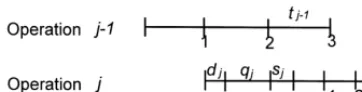
Fig. 1. Increment to the manufacturing cycle time, ift
j)tj~1
andq
j#sj#(Q!1)(tj!tj~1))0.
Table 1
Schedule of operationjfor a 3-unit lot
Unit 1 Unit 2 Unit 3 Completion time at operationj!1 6 12 18 Earliest available time at operationj 7 13 19 Earliest start time at operationj 14 16 19 Earliest"nish time at operationj 16 18 21
the idle time forward in such a way that machinejis available for the Qth unit exactly at the time it arrives from stage j!1. The transport time, wait-ing time, and setup time could occur any time before the processing time of the "rst unit. This situation in which all the idle time is pushed for-ward is shown for a 3-unit lot in Fig. 1. Example 1 provides a numerical illustration.
Example 1.
Lett
j"2(minutes),tj~1"6(minutes),dj" 1(min-ute),q
j"5(minutes),sj"2(minutes), andQ"3, then q
j#sj#(Q!1)(tj!tj~1)"!1(0. According to
our formula, the incremental manufacturing cycle time at this stage is d
j#tj"3 minutes. Suppose the "rst unit starts operation j!1 at time zero. Table 1 shows how the operations take place at stagej. Note that the earliest start time at operation j for Unit 1 is the completion time of the unit at operationj!1 plus (d
j#qj#sj). For Units 2 and 3, the earliest start time at operationj equals the maximum of the earliest available time at operation jfor the unit and the earliest"nish time at opera-tionjfor the previous unit.
From the last two lines of Table 1, we see that if we start operationjfor all the sub-lots as soon as the sub-lots are available, there will be 1 min idle time between the second and third sub-lots. To satisfy the assumption that no idle time exists be-tween consecutive sub-lots on the same machine, we delay operationjfor the"rst sub-lot from time 14 to time 15. Thus, Unit 1 will be"nished at time 17, Unit 2 at time 19, and Unit 3 at time 21.
We make a few remarks about the above case. First, the increment in the manufacturing cycle time is always the same, i.e., *¹
j"dj#tj, no matter where we put the idle time. Second, where we put the idle time will make a di!erence in the calcu-lation of *¹
j#1 when the processing time for
operationj#1 is larger than the processing time for operationj. We have made the assumption that all idle time is moved backwards before starting the operation, which is defensible because in practice it is desirable to keep the machine continuously busy after initiating production of a lot. Third, the assumption of no idle time between consecutive sub-lots holds for all cases, although in some ex-treme situations, this could mean excessive idle time at some stages. For example, consider a two-stage process with a lot size of two units. Let us say that the processing time at the"rst stage is 90 min-utes per unit and that at the second stage is only 1 minute. Suppose we adopt lot streaming with a sub-lot size of one unit. The assumption of no idle time between consecutive sub-lots would mean an idle time of 89 minutes at the second stage. How-ever, the total time for processing the lot through the two-stage process, i.e., the manufacturing lead time is 181 minutes, whether we allow or disallow idle time between sub-lots. Thus our analysis holds. Also, in such situations, allowing for no idle time between sub-lots in such cases, may indeed be more desirable. This is because in a deterministic envi-ronment, a larger chunk of idle time allows the managers greater #exibility in accommodating other jobs that could be completed within the idle time at the second stage. Finally, in our analysis units are recognized as WIP from the moment a lot enters the "rst stage and until it leaves the "nal stage as"nished goods. Thus, the holding cost for WIP is fully accounted for in our model even when there is a large idle time in some extreme cases like the one in the above hypothetical example.
(b) If q
j#sj#(Q!1)(tj!tj~1)'0, which
Fig. 2. Increment in the manufacturing cycle time, ift
j)tj~1
andq
j#sj#(Q!1)(tj!tj~1)'0.
Table 2
Schedule of operationjfor a 3-unit lot.
Unit 1 Unit 2 Unit 3 Completion time at operationj!1 6 12 18 Earliest available time at operationj 7 13 19 Earliest start time at operationj 14 17 20 Earliest"nish time at operationj 17 20 23
Fig. 3. Increment in the manufacturing cycle time ift
j'tj~1.
Table 3
Schedule of operationjfor a 3-unit lot
Unit 1 Unit 2 Unit 3 Completion time at operationj!1 2 4 6 Earliest available time at operationj 3 5 7 Earliest start time at operationj 10 16 22 Earliest"nish time at operationj 16 22 28
*¹
j"
G
(1!Ij)(dj#tj)#Ij(qj#sj#(Q!1)(tj!tj~1)),∀j3A,
(1!I
j)(dj#qj#sj#Qtj!(Q!1)tj~1)#Ij(qj#sj#dj#Qtj!(Q!1)tj~1),∀j3B.
incremental manufacturing cycle time is
*¹
j"dj#qj#sj#Qtj!(Q!1)tj~1.
The case for a 3-unit lot is illustrated in Fig. 2. It is followed by a numerical example.
Example 2. We use the same parameters as in
Example 1, except that t
j"3(minutes). Now, we have q
j#sj#(Q!1)(tj!tj~1)"1'0. The
in-cremental manufacturing cycle time at this stage is d
j#qj#sj#Qtj!(Q!1)tj~1"5 minutes and
the operations taking place at stagejare shown in Table 2.
4.2. Scenario 2: t
j'tj~1
In this scenario, a sub-lot from operationj!1 is always available whenever machine j is available and therefore there is no idle time on machine j.
The incremental manufacturing cycle time is
*¹
j"qj#sj#(Q!1)(tj!tj~1)#tj#dj. The case for a 3-unit lot is illustrated in Fig. 3. It is followed by a numerical example.
Example 3. We use the same parameters as in
Example 1, except that t
j"6(minutes), tj~1"
2(minutes). The incremental manufacturing cycle time at this stage isq
j#sj#(Q!1)(tj!tj~1)#
t
j#dj"22 minutes. The schedule of the opera-tion at stagejis shown in Table 3.
4.3. A generalization
Let
I j"
G
1, ∀t
j'tj~1,
0, ∀t
j)tj~1,
and
A"Mj:q
j#sj#(Q!1)(tj!tj~1))0N,
B"Mj:q
j#sj#(Q!1)(tj!tj~1)'0N.
The calculations for *¹
j under di!erent scen-arios can be generalized as follows:
Note that if j3A, then t
j)tj~1, and therefore
I
j"0. Therefore,
*¹
j"
G
dj#tj,∀j3A, d
Summation of*¹
j over all scenarios, yields the manufacturing cycle time:
In practice, we move the whole lot or sub-lots rather than individual units between operations. If Q units are produced as a lot and divided into bsub-lots of equal size, we can treat each sub-lot as one unit. Thus, we obtain the following result:
¹ order under processing. The processing of each order will be started Q/D time units prior to the time at which Q units of the "nished item are required. In a deterministic setting, there is no problem if more than one order is outstanding because each order will arrive in the exact time sequence in which it is placed. In line with the traditional inventory modeling approach, our model recognizes the relevant costs over a unit time interval, i.e., one year. Consequently, the feasibility of our model in a deterministic environment with no capacity constraints is always assured.
Having thus determined the manufacturing cycle time, ¹
m, we visualize inventory process and the build-up and the depletion of the WIP as follows. A batch of Q units of the"nished item leaves the
"nal operation at the end of each production cycle of length Q/D time units thereby satisfying the demand with no shortages or backorders. For this batch,Qunits of raw materials will enter processing at the"rst operation,¹
mtime units prior to the end of the production cycle to allow for the manufac-turing lead time. WIP starts with zero at the
begin-ning of a manufacturing cycle. Q units enter into WIP uniformly over a timet
1, the processing time
for operation 1, continue as WIP undergoing pro-cessing at the subsequent operations, and then start leaving the WIP at a uniform rate beginning at a timet
mprior to the end of the cycle at time¹m. Thus, the expression for the time-weighted work-in-process will be
IT"Q¹
m!Q2(t1#tm)/2. (4)
5. Optimization models and computational results
The expression for the total relevant cost (TRC) includes the costs associated with setup, transpor-tation, and holding of WIP and"nished goods and can be written as
TRC(Q,b)"AD/Q#GbD/Q
#Q(1!Dt
m)h1/2#h2D*IT/Q. (5)
By substituting (1) and (4) into (5), we get
designed to operate at nearly equal production rates. The second case represents the situations in which the size of the transfer batch or, equivalently, the number of sub-lots is "xed by the size of the pallets or containers used to move items.
5.1. A special case:Identical production rates at all stages
When the production rates at all the stages are identical, the processing times t
j are same for all operationsj. Settingt
j"t, for all j, expression (6) can be simpli"ed to
TRC(Q,b)"AD/Q#GbD/Q#Q(1!Dt)h
1/2
#h
2D
A
m + j/2
(d
j#qj#sj)
#(m!1)tQ/b
B
. (7)Letb"Q/Q@. Then,
TRC(Q,Q@)"AD/Q#GD/Q@#Q(1!Dt)h
1/2
#h
2D
A
m + j/2
(d
j#qj#sj)
#(m!1)tQ@
B
. (8)By setting
LTRC(Q,Q@)
LQ "0, we getQH"
S
2AD (1!Dt)h1
. (9)
By setting
LTRC(Q,Q@)
LQ@ "0, we getQ@H"
S
G h2(m!1)t
. (10)
Because
L2TRC(Q,Q@) LQ2 "
2AD Q3 '0,
L2TRC(Q,Q@) LQ@2 "
2GD
Q@3'0, and
L2TRC(Q,Q@) LQQ@ "0,
the Hessian matrix is positive de"nite and therefore TRC(Q,Q@) is a convex function. This guarantees the existence of a global minimum for TRC at (QH,Q@H).
We see that when the production rates are the same for all machines in a multi-stage production system, the optimal production lot is exactly the same as in the economic lot quantity model pro-posed by Eilon [4] in which the WIP is ignored. Since TRC(Q,Q@) is a convex function, we can"nd the optimal integer solution (QHH,Q@HH) by compar-ing the total relevant costs for the points (Q,Q@) in the neighborhood of (QH,Q@H) that satisfy the condi-tion thatQ,Q@, andQ/Q@are all integers. There exist a"nite number of such points and the optimal lot and sub-lot sizes are the ones that give the smallest total relevant cost.
We observe that the optimal lot and sub-lot sizes in (9) and (10) do not depend on the waiting times, which in the MRP tradition have been assumed to be independent of the lot size. From this observa-tion, we derive the obvious (nevertheless quite signi"cant implication for policy implementation) insight that these optimal lot and sub-lot sizes will be valid even if waiting times at the di!erent stages of a multistage manufacturing system are uncertain as Graves and Kostreva [8] obtained for the two-machine system.
5.2. More general case:Production rates not identi-cal at all stages but b isxxed
We present the analysis of this general case by examining two situations: (1) the simpler situation when b"1, and (2) the more general situation whenb'1.
5.2.1. The situation whenb"1
Whenb"1, i.e., the transfer batch size is equal to the production batch size the total cost expres-sion (6) simpli"es to
TRC(Q)"AD/Q#GD/Q#Q(1!Dt m)h1/2
#h
2D
A
Qm + j/1
t
j!(t1#tm)Q/2
#+m
j/2
(q
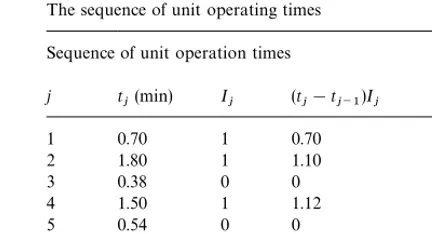
Table 4
The sequence of unit operating times Sequence of unit operation times
j t
j(min) Ij (tj!tj~1)Ij (sj#qj)
1 0.70 1 0.70 75
2 1.80 1 1.10 115
3 0.38 0 0 475
4 1.50 1 1.12 25
5 0.54 0 0 774
6 0.20 0 0 147
7 1.40 1 1.20 39
8 0.30 0 0 375
9 0.48 1 0.18 25
By setting dTRC(Q)/dQ"0, we get
EPL"
S
2(A#G)D(1!Dt
m)h1!h2D(t1#tm)#2h2D+mj/1tj . (12)
Because d2TRC(Q)/dQ2"2(A#G)D/Q3'0, TRC(Q) is convex, and is minimized byQ"EPL.
5.2.2. The situation when b'1
To analyze this case, we decompose expression (6) for the total relevant cost into two parts, TC
1(Q)
and TC
2(Q):
TC
1(Q)"AD/Q#GbD/Q#Q(1!Dtm)h1/2
!h
2DQ(t1#tm)/2, (13)
TC
2(Q)"h2D
A
Q/bA
+j|A{
t j#+
j|B{
t j~1
B
#+
j|B{
(q
j#sj#Qtj!Qtj~1)
#+m
j/2
djB, (14)
andA@andB@are as de"ned in (2) and (3). The mathematical analysis of these equations is complex and closed form solutions are intractable. It is therefore necessary to use an algorithmic numerical search procedure to "nd the optimal solutions. When the transportation cost is invari-ant to the number of sub-lots, then, it is clearly evident that TC
1(Q) is a well-behaved function for
numerical search. As Graves and Kostreva [8] point out, a constant cost for transportation is simple and adequate for most circumstances. The analysis would hold even if the transportation cost involves a constant plus a convex function of the transfer lot size. In Appendix A, we show that TC
2(Q) is a piece-wise linear function with
increas-ing slopes and therefore it is also a well-behaved function. Thus, the sum of TC
1(Q) and TC2(Q) is
also a well-behaved mathematical function that accommodates a numerical search to seek the opti-mum, although it is not di!erentiable at a "nite number of points.
From (2) and (3), ift
j~1)tj, thenj3B@. De"ne a setCasC"Mj:t
j~1'tjNandA@is a subset ofC.
Rank the values of (q
j#sj)b/(tj~1!tj)(b!1) for alljinCin an increasing order. LetN[i] be theith number in the ordered series, whereitakes on the values 1, 2,2,DCD, andDCDis the number ofj@s inC.
Then N[1], N[2],2, and N[DCD] re the points
where Eq. (6) is not di!erentiable. LetQ@
i,i"1, 2,2,DCD#1, be the saddle points (where the"rst derivative of Eq. (6) is zero) for the intervals [0, N[1]), [N[1], N[2]),2,[N[DCD], #R), respectively. Note that someQ@
is may not be feasible (i.e., outside the corresponding interval). In Appendix B, we show that Q@
i decreases with in-creasingi. This property and the nature of the total relevant cost function facilitate the search for the optimal value. The following algorithm is used to
"nd the optimalQHwhen we do not requireQHto be an integer multiple ofb. We then look for the integer solution in the neighborhood ofQHto ob-tain the minimum cost solution.
Computational Algorithm Step 1. If Q@
@C@`1 is feasible, then Q@@C@`1 is the
optimal value and stop. Otherwise, leti"DCD, and go to step 2.
Step 2. If N[i!1])Q@
i(N[i], then Q@i is the optimal value and stop. IfQ@
i*N[i], thenN[i] is the optimal value and stop. If Q@
i(N[i!1], let i"i!1 and go to the beginning of step 2.
5.3. Computational results}comparison of total relevant costs
Q@5"
S
2(A#bG)D(1!Dt
m)h1!h2D(t1#tm)#2h2D((+j/M3,5,6,8Nt
j#+j/M1,2,4,7,9Nt
j~1)/b#+j/M1,2,4,7,9N(t
j!tj~1))
"5203(units).
numerical example. We set the parameter values as follows: D"50,000 units per year, A"$220 per setup,G"$20 per sub-lot,h
1"$0.40 per unit per
unit time, h
2"$0.24 per unit per unit time. We
assume 250 working days per year and 480 minutes per working day. The sequence of processing stages, and the sum of setup times and wait times at each stage of manufacturing are given in Table 4. Without loss of generality, the transportation times,d
j, have been assumed to be zero.
5.3.1. Application of the traditional ELQ model
In this approach, the production lot size is deter-mined based on the "nal stage of the operations using the formula (see, [4]):
S
2AD(1!Dt m)h1
.
Using the data in this example,
ELQ"
S
(2)(220)50,000(1!50,000M0.48/(480)(250)N)0.4"8292.
This lot size of 8292 units is used for processing at each stage. The total annual cost including the carrying costs associated with WIP inventory is given by
TC
ELQ"AD/Q#Q(1!Dtm)h1/2
#h2DQ[t
j!(t1#tm)/2].
For the data in this example and a lot size of 8292 units, the total cost is$8619.33.
5.3.2. Application of our EPL model withb"1 In this approach, which takes into WIP costs but no lot streaming, the optimal lot size, EPL, is deter-mined using our model or the Eq. (12). For the data in this example, EPL works out to 4523 units. The total annual cost including the carrying costs
asso-ciated with WIP inventory is given by Eq. (11). For the data in this example and a lot size of 4523 units, the total cost works out to$6675.69.
5.3.3. Application of our EPL model with b"5
In this approach, which takes into WIP costs and lot streaming, the optimal lot size, EPL, is deter-mined using our algorithmic procedure as outlined in the steps below.
1. Determine the set C. Because C" Mj:t
j~1'tjN, we haveC"M3, 5, 6, 8N. 2. Calculate (q
j#sj)b/(tj~1!tj)(b!1) for all j in C. The values of (q
j#sj) are 475(minutes), 774(minutes), 147(minutes), and 375(minutes) when j"3, 5, 6, and 8, respectively. The corresponding values of (q
j#sj)b/(tj~1!tj)(b!1) forj"3, 5, 6, 8 are 418, 879, 919, and 426. The non-di!erentiable points for the total cost function areN[2]"418, N[4]"426,N[10]"879, andN[9]"919.
3. ForQ(418,j"3, 5, 6, 8 all belong toB@; for 418)Q(426,j"3 belongs toA@, the rest belong-ing toB@; for 426)Q(879,j"3, 8 belong toA@, while the rest belong to B@; for 879)Q(919, j"3, 5, 8 belong toA@, while j"6 belongs toB@; whenQ*919, j"3, 5, 6, 8 all belong to A@. The optimalQ when j"3, 5, 6, 8 all belong to A@ is given by
SinceQ@
5'N[4], it follows from the algorithm that
Q@
5is the optimal value when we relax the condition
thatQ@5 must be an integer multiple ofb. Since the number of sub-lots,b, is 5 and the lot size 5203 is not an integer multiple of 5, we compare the total relevant costs for the appropriate neighboring pointsQ"5200 andQ"5205. The optimal value is QH"5205 because it gives the smaller total relevant cost,$6150.
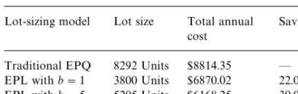
The results for the numerical example are sum-marized in Table 5 below.
Table 5
Summary of computational results
Lot-sizing model Lot size Total annual cost
Savings
Traditional EPQ 8292 Units $8814.35 * EPL withb"1 3800 Units $6870.02 22.05% EPL withb"5 5205 Units $6168.25 30.02%
annual cost can be achieved relative to the tradi-tional approach in which the lot size is determined using the ELQ model for the "nishing stage only. Although the exact savings are context- and data-dependent, the computational analysis demon-strates the potential for cost savings from the application of our lot-streaming model.
6. Conclusions
In this paper, we have presented a rigorous ap-proach to compute the manufacturing cycle time for an item in a multistage production system when lot streaming is applied so that the costs associated WIP inventory can be recognized appropriately in determining the optimal production lot size. We developed expressions for the total cost taking into account the costs associated with setup, transporta-tion, and carrying both the WIP and"nished prod-uct inventory and, then discussed procedures to
"nd the optimal production lot size that minimizes the total cost. Through computational analysis we demonstrated the potential for substantial cost sav-ings from the application of our lot-streaming model relative to the namKve, traditional approach in which the lot size is determined using the ELQ model for the"nishing stage only.
In terms of the contributions to the modeling of inventory systems, our paper has endeavored to take a modest step toward the development of a more general inventory model for a single item in the context of a multistage manufacturing system incorporating the cost of work in process inven-tory. Our methodology and the model we have presented deal with re"nements to the models currently in the literature and make two speci"c contributions. First, our model is more realistic in that it captures more accurately the components of
the manufacturing lead time that are encountered in a multistage production/inventory system. Clearly, managers will"nd it more realistic to as-sign values the time required for setup, moving, and planned delay at each stage of a multistage produc-tion system compared to using a multiplier to com-pute the manufacturing lead time from the technological processing time. Furthermore, the estimation or guessing of the multiplier is prone to serious errors especially in MRP systems. As Graves and Kostreva [8] point out `it is not un-heard of, for example, to have a standard MRP lead time of several months while actual production lead time runs approximately one weeka. Second, our model facilitates the application of lot streaming to multistage systems MRP by going beyond the cur-rently available models for two-station systems and o!ering a generalization to any multistage produc-tion systems.
In terms of the contributions from a managerial perspective, our model can lead to signi"cantly better cost performance as we have demonstrated through numerical examples, especially when the manufacturing lead time is large compared to the technological processing time as is commonly encountered in practice.
Finally, for future research, we would like to explore the total cost performance of the di!erent lot sizing approaches using di!erent values for b, i.e., the number of sub-lots in the context of a more detailed factorial experimental design with several di!erent levels of the cost and demand parameters.
Appendix A
Proof. (TC
2(Q) is a piece-wise linear function with
increasing slopes).
Since
TC
2(Q)"h2D
A
Q/bA
+j|A{
t j#+
j|B{
t j~1
B
#+
j|B{
(q
j#sj#Qtj!Qtj~1)
#+m
j/2
Q@
2(Q) has"nite breakpoints
and within any consecutive breakpoints TC
2(Q) is
a linear function.
At any breakpoint, Q
j"(qj#sj)b/(tj~1!tj) (b!1), wherejis an element in the setC. We shall
prove that TC
2(Q) is actually continuous at the
pointQ j.
For any pointjinC, the di!erence between the right-hand limit and the left-hand limit of TC
2(Q)
2(Q)is continuous at all breakpoints. To
prove that the lines have increasing slopes, we con-sider the change of the slope at pointiinC. When Q(Q
then the new line has a slope of
h
Hence the change of the slope at the breakpoint is
h
Proof. (Saddle point, Q@
i, is decreasing in i). By using the Eqs. (13) and (14), the saddle pointQ@
i of the total cost function forN[i!1])Q(N[i] is
Letj
i"(+j|A{tj#+j|B{tj~1)/b#+j|B{(tj!tj~1).
Note that Q@
i becomes smaller when ji becomes larger. From the proof in Appendix A, it is known thatj
i is increasing withi, and hence the proof is complete. h
References
[1] F.R. Jacobs, D.J. Bragg, Repetitive lots: Flow-time reduc-tions through sequencing and dynamic batch sizing, Decision Sciences 19 (1988) 281}295.
[2] K.R. Baker, D.F. Pyke, Solution procedures for the lot-streaming problem, Decision Sciences 21 (1990) 475}491. [3] D.H. Kropp, T.L. Smunt, Optimal and heuristic models for lot splitting in a#ow shop, Decision Sciences 21 (1990) 691}709.
[4] S. Eilon, Elements of Production Planning and Control, Macmillan, New York, 1962, 227}263.
[5] H.A. Taha, R.W. Skeith, The economic lot sizes in multi-stage production systems, AIIE Transactions 2 (1970) 157}162.
[6] A.L. Szendrovits, Manufacturing cycle time determination for a multistage economic production quantity model, Management Science 22 (1975) 298}308.
[7] S.K. Goyal, Economic batch quantity in a multistage pro-duction system, International Journal of Propro-duction Research 16 (4) (1978) 267}273.
[8] S.C. Graves, M.M. Kostreva, Overlapping operations in material requirements planning, Journal of Operations Management 6 (1986) 283}294.
[9] S.C. Graves, A tactical planning model for a job shop, Operations Research 34 (1986) 22}533.