Directory UMM :Data Elmu:jurnal:J-a:Journal Of Applied Geophysics:Vol44.Issue4.2000:

www.elsevier.nlrlocaterjappgeo

Parallel finite element algorithm with domain decomposition for

three-dimensional magnetotelluric modelling

Fabio I. Zyserman

a,)

_{, Juan E. Santos}

b,c

a

Departamento de Fısica, Uni´ Õersidad Nacional de La Plata, C.C. 67, 1900 La Plata, Argentina

b

CONICET, Departamento de Geofısica Aplicada, Fac. de Cs., Astronomicas y Geofısicas, U.N.L.P., Paseo del Bosque s´ ´ ´ rn, 1900 La Plata, Argentina

c

Department of Mathematics, Purdue UniÕersity, West Lafayette, IN 47907, USA

Received 13 July 1999; accepted 9 March 2000

Abstract

Ž .

We present a new finite element FE method for magnetotelluric modelling of three-dimensional conductivity structures. Maxwell’s equations are treated as a system of first-order partial differential equations for the secondary fields. Absorbing boundary conditions are introduced, minimizing undesired boundary effects and allowing the use of small computational domains. The numerical algorithm presented here is an iterative, domain decomposition procedure employing a nonconform-ing FE space. It does not use global matrices, therefore allownonconform-ing the modellization of large and complicated structures. The algorithm is naturally parallellizable, and we show results obtained in the IBM SP2 parallel supercomputer at Purdue University. The accuracy of the numerical method is verified by checking the computed solutions with the results of COMMEMI, the international project on the comparison of modelling methods for electromagnetic induction. q₂₀₀₀ Elsevier Science B.V. All rights reserved.

Keywords: Magnetotelluric methods; Numerical models; Finite element analysis; Electromagnetic field; Conductivity

1. Introduction

Numerical modelling of three-dimensional con-ductivity structures in the earth has experienced a rapid development during the last few years. There are three types of methods that are mostly used,

Ž .

namely integral equation IE methods, finite

differ-)_{Corresponding author. Fax:}

q54-221-4252006.

Ž E-mail address: zyserman@venus.fisica.unlp.edu.ar F.I.

Zy-.

serman .

Ž . Ž .

ence FD methods and finite element FE methods. Among the contributors to the former, we can

men-Ž .

tion Wannamaker 1991 , who extended the capabili-ties of the integral method to deal with complicated

Ž .

models; Xiong 1992 proposed an iterative method with block partitioning to reduce memory and

stor-Ž .

age requirements; and Zhdanov and Fang 1996 introduced a quasi-linear approximation for the inte-gral method. The FD has been studied, for example,

Ž .

in Mackie et al. 1993 who solved the integral form of Maxwell’s equations, assigning the tangential magnetic field as boundary condition. For the FE,

Ž .

Mogi 1996 used hexahedral elements to calculate

0926-9851r00r$ - see front matterq_{2000 Elsevier Science B.V. All rights reserved.}

Ž .

the secondary fields, and employed asymptotic boundary conditions.

Ž .

More recently, Zhdanov et al. 1997 presented the results from COMMEMI where different meth-ods of the three classes mentioned above compare their results for standard test models; among them,

Ž

only one was a FE. It is well-known Mackie et al.,

.

1993 that FE can more accurately solve complicated structures than IE but up to now it has, for the three-dimensional case, the iron constraint of huge memory requirement for the storage of the global matrices needed to obtain the results.

In the present work, we introduce a hybridized nonconforming iterative domain decomposed mixed

Ž . Ž

finite element procedure DDFE Douglas et al.,

.

2000 to solve Maxwell’s equations treated in the form of a system of first-order partial differential equations for the scattered electric and magnetic fields. The boundary conditions employed are

first-Ž .

order absorbing ones Sheen, 1997 , which allow for a significant reduction in the size of the computa-tional domains and are easily introduced into the algorithm. Undesired effects generated by the artifi-cial boundaries, such as reflections, are diminished by these boundary conditions. Besides, because of the domain decomposition approach, no global ma-trices need to be constructed and only 12=12 linear systems or block diagonal linear systems are solved at each iteration level in each of the subdomains in which the studied region is divided; this feature in turn makes storage requirements smaller. Finally, we mention that the design of the proposed procedure leads to a very efficient parallel code, requiring a small flow of information among processors during the calculations.

In Section 2, we present the model and the differ-ential problem to be solved, and afterwards, we introduce the numerical method. Finally, we show some results of our DDFE, comparing them with

Ž .

those compiled in Zhdanov et al. 1997 and draw the conclusions.

2. The forward differential model

Recall that if E and H denote, respectively, the electric and magnetic fields for a given angular

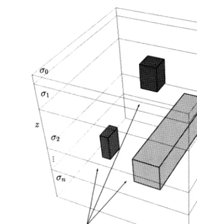
Fig. 1. The 3-D model.

frequency v, then the time harmonic Maxwell’s equations in a region free of sources state that

==HssE,

Ž .

1a

==EsyivmH ,

Ž .

1b

where s and m denote the electrical conductivity and magnetic permeability, respectively and as it is usual in magnetotellurics, displacement currents have

Ž .

been neglected. Also, associated to Eqs. 1a and

Ž1b , we have the consistency conditions imposing.

the continuity of the tangential electric and magnetic fields and the continuity of the current density and magnetic flux normal to any interior interface. Let us

Ž . Ž .

consider Eqs. 1a and 1b in the three-dimensional domain V shown in Fig. 1. The uppermost layer of

V represents the air, while the others represent a horizontally layered earth with any number of arbi-trarily shaped embedded inhomogeneities. The latter must not necessarily lie within a single layer of the former.

According to the description of our domain, the electrical conductivity distribution has the form:

Ž

In analogy with the 2D case Wannamaker et al.,

.

1987; Zyserman et al., 1999 , we will formulate the differential model in terms of scattered fields. Let the primary electromagnetic fields E and H be physi-p p

Ž .

cally meaningful solutions of Maxwell’s Eqs. 1a

Ž .

and 1b for the horizontally layered model with

Ž .

s_ss_p z . Then, let E_tsE_pqE and H_{s ts}H_pqH_s

denote the total electromagnetic fields in V with

Ž .

conductivity s as in Eq. 2 induced by a plane, monochromatic electromagnetic wave of frequency

v incident upon its top boundary. Finally, let E ands

H be the scattered electromagnetic fields due to thes

presence of the conductivity anomalies Vi; they satisfy the equations

sEsy==HssysiEpsyF ,

Ž .

3a

ivmHsq==Ess0.

Ž .

3b which are the ones we are going to deal with. In order to minimize the effect of the artificial bound-aries, we will use the absorbing boundary condition

Ž .

introduced by Sheen, 1997 :

1yi P aEqn=H s0 onEV'G, 4 simplicity, from now on we will omit the subscripts for the secondary fields.

Let us briefly comment on the meaning of Eq.

Ž .4 . Our aim is to simulate, as close as possible, the vanishing of the electromagnetic field at infinity, but considering a finite domain. On choosing, e.g., a Dirichlet boundary condition on G, one must extend the domain until the fields are negligible, leading to the use of large computational domains at the cost of increasing CPU times and memory requirements. On

Ž .

the other hand, by using Eq. 4 , we make a field normally ‘arriving’ to the borderG to be ‘absorbed’ by it, i.e., we make it leave our domain with no reflections; and this can be done relatively close to the inhomogeneities.

Next, we proceed to describe the domain

decom-position procedure. Let us consider a partition of our

original domain V into non-overlapping — not necessarily homogeneous — parallelepipeds Vj of volume hxj=hyj=h , jzj s1, . . . , J. Let Gj be the boundary of the subdomain Vj, consisting of six

rectangles, namelyG_s FF_ront, BB_ack,WW_est, EE_ast,

j

4 Ž

N

N_orth, SS_{outh to avoid cumbersome notation, the}

subindex j associated with each rectangle in Gj is

. Ž . Ž .

Here B stands for the intersection of the bound-j

ary of the domain Vj with G. Clearly, consistency conditions need to be imposed on all interior

bound-Ž

aries; i.e., on all rectangles building Gj such that

.

their intersection with G is empty . The natural conditions are given, as already stated, by the conti-nuity of the tangential electric and magnetic fields on these boundaries:

nj=Hjsynk=Hk onGjk,

Ž .

7a

P Et jsP Et k onGjk.

Ž .

7b In the above equations Gjk stands for the face shared by the adjacent domains Vj and Vk. Of course, G_jksG_{k j}, but care must be taken when considering the direction of the normal vector to the face, i.e., G_jk is the face as seen from V_j and G_{k j} is the same face but as seen from V_k. For the iterative algorithm to be defined below, it is more convenient

ŽDouglas et al., 1993 to replace Eqs. 7a and 7b. Ž . Ž .

by the equivalent Robin-type transmission condi-tions:

n_j=H_jsyn_k=H_kyb_jk

Ž

P Et jyP Et k

.

onGjk_;Gj,

Ž .

8a

nk=Hksynj=Hjybjk

Ž

P Et kyP Et j

.

onGk j_;Gk,

Ž .

8b

Here, bjk is a complex parameter defined on the interfaces Gjk with a positive real part and a nega-tive imaginary part. In Appendix A, we explain how we chose its values.

Ž .

To obtain a variational formulation for Eqs. 5 –

Ž .6 , we proceed as usual ŽDouglas et al., 1997;

. Ž .

Martinec, 1997 . We test Eq. 5a with real vector

Ž . Ž .

functions w x, y, z such that==w x, y, z is square

Ž .

integrable; and Eq. 5b by square integrable real

Ž . Ž .

Using integration by parts in the terms involving the curl of the magnetic field, and applying the Robin

Ž . Ž .

transmission boundary conditions 8a and 8b for the interior boundaries and the absorbing boundary

Ž .

condition 6 on B , we obtain the equations:_j

sEwd3_x

The sum in the third term in the left-hand side of the first equation runs over the rectangles G_jk build-ing the interface among Vj and its neighbours; whenever Gjk is also part of G, the contribution of the corresponding integral is neglected. On the other hand, the contribution of the last term on the left-hand

Ž .

side of Eq. 9a is different from zero only when the integration is done on a rectangle that is simultane-ously part of the boundary of the computational domain V.

The idea of the domain decomposition procedure is to solve the posed problem separately in each

Ž .

subdomain Vj. Taking into account that Eqs. 8a

Ž .

and 8b involves only subdomains adjacent to V_j, we propose the following iterative algorithm:

Ž 0 0_.

1. Choose initial values E , H

Ž nq1 nq1_.

We point out that for the subdomain Vj, the

Ž .

right-hand side of Eq. 10a contains unknowns be-longing to its neighbour cells, and they are one iteration step behind, i.e., they are assumed to be data at the current iteration level. In Section 3, we will define the discrete procedure motivated by the above iteration.

3. The finite element procedure

In order to simplify the description of the numeri-cal procedure, we will assume that the domain

de-Ž

composition partition the already mentioned

par-.

alellepipeds Vj of the domain V coincides with the FE partition. Later, we will briefly indicate the changes for the case in which the subdomains consist of strips in the x-direction.

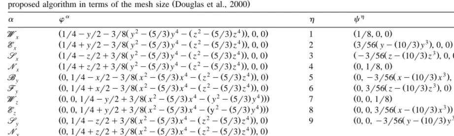
In each cell Vj, we approximate the electric and magnetic fields, respectively, by the expressions:

2 x 2 y 2 z

where the superscripts a andh cover all the corre-sponding basis functions given in Table 1, and the complex coefficients ´a, nq1

and hh, nq1 need to be

j j

determined at the iteration level nq1. Therefore, we use 12 basis functions for E and nine basis_j functions for H . The scaling and translation of the_j

a h _{Ž .}

basis functions w and c in Eq. 11 is made in order to keep the variables within the reference

w x3

element y1,1 . In Fig. 2, the reference cube and relation among coefficients belonging to adjacent paralellepipeds is shown. The dependence of the lengths h , hx y and h on the index j was omittedz

Table 1

w x3_{Ž .}

The nonconforming FE basis functions for E and H, defined in _y1,1 see Fig. 2 for details on the reference cube . Let us consider, to clarify ideas, the first basis function for the electric field. The only nonzero component of this vector function, i.e., the x-component, takes the value 1 on the mid-point of theWW _{face, and zero on the mid-points of all other faces. The other basis functions display similar}

behaviour. It can also be seen that the space spanned by the functionsch _{is the curl of the one spanned by the functions w}a_{, as usual}

requirement for mixed methods. The selected basis functions also make it possible to obtain as estimate on the rate of convergence of the

Ž .

proposed algorithm in terms of the mesh size Douglas et al., 2000

a h

The next step is to hybridize Arnold and Brezzi,

.

1985 the algorithm to make the algebraic problem easier. This is achieved by eliminating the constraint requiring the continuity of the tangential components of the electric field on the faces G_jk, and enforcing instead the required continuity through Lagrange multipliers defined at the interelement boundaries

Gjk. Furthemore, as an additional simplification, in-stead of applying the continuity of these tangential components on the whole interface Gjk, we will impose it only at the mid-points mjk of Gjk. The introduction of the Lagrange multipliers allows for a simplification of the associated algebraic problem, which becomes block diagonal and consequently, the approximate electric and magnetic fields can be sep-arately computed. Thus, for each one of the rectan-gles building G_j that are not part of the boundaryG, we introduce a two-dimensional constant vector or Lagrange multiplier lnq1 _{associated with the value}

jk

of n =Hnq1 _{at the mid-point m of the face G ,}

j j jk jk

i.e., we will have an additional two-dimensional unknown vector lnq1 _{per each face of the domain}

jk

Note that as stated above, Eq. 12 imposes the continuity of the tangential components of the elec-tric field only at the mid-points m_jk of the faces G_jk. Also, accordingly with what we just mentioned, the expression n =Hn _{in the last integral of the}

right-k k

Ž .

hand side of Eq. 10a is replaced by the Lagrange multiplier ln_.

k j

Ž . Ž .

To get the algebraic form of Eqs. 10a – 10c , the

Ž .

fields E and H as defined in Eq. 11 are replacedj j

Ž . Ž . a

in Eqs. 10a and 10b . Then, the functions w and

h _{Ž .}

c scaled as in Eq. 11 are taken as test functions

Ž . Ž .

in Eqs. 10a and 10b , respectively, in the order given in Table 1. The surface integrals in Eqs.

Ž10a – 10c. Ž . were approximated by the mid-point < < Ž . Ž .

rule, i.e., we used HAfgd Sf A f m g m , where

<A is the area of the surface A, and m is its< mid-point.

This task yields a 21=21 linear system of equa-tions for each subdomain V_j, at each iteration level. The problem can be further simplified because the choice of the basis functions for the magnetic field allows to get the coefficients hh, nq1 _{in terms of the}

j

coefficients ´a, nq1_{, by using the set of linear}

equa-j

Ž .

tions rendered by Eq. 10b . Once this simple alge-bra is carried out, we end up with a 12=12 linear system of the form C ´nq1

sbn_{. The coefficient}

j j j

matrices C remain unchanged along the iterativej

Ž . w x3

Fig. 2. a Display of the reference cube y1, 1 . We associate the coefficients of the electric field with the mid-points of the faces of the cube, where the single nonzero component of the respective basis functions takes the value 1. The degrees of the freedom of H are obtained

Ž .

from momenta, therefore there is no specific position associated with them in the reference cube. b Continuity of the electric field is asked,

Ž .

as stated in Eq. 12 , only in the mid-point mjkof the face. Displayed coefficients´, which are the only ones involved in this interface,

Ž . ´x WWx ´t WWz

asymptotically verify this condition. Also, because of Eq. 12 , we have that the equations lj _sylk and lj _sylk hold asymptotically, or equivalently, we have continuity of the tangential components of the magnetic field at the mid-point of the interface asymptotically. Similar is the situation for the other faces.

explicitly shown. The last task is to get the discrete

Ž .

version of Eq. 12 , which is easily accomplished

Ž .

using Eq. 11 .

We can therefore state our iterative algorithm as follows:

Ž a,0 0_.

1. Choose initial values ´j , ljk for the un-knowns in all cells Vj.

2. For all domains V_j

Solve the 12=12 linear system for the un-knowns ´a, nq1

.

j

Compute lnq1

.

jk

3. Check for convergence. If it has not been achieved, go to step 2.

As is usual for iterative algorithms, convergence is reached when the relative error of the calculated coefficients is smaller than a prescribed tolerance, i.e., when within this tolerance the coefficients have stopped changing. At this stage, the unknowns hh_j can be easily calculated as indicated above.

We note that the convergence of the above itera-tive procedure to the solution of the original

differen-Ž . differen-Ž .

tial problems 3 – 4 has been demonstrated in

Dou-Ž .

glas et al. 2000 . More specifically, in the men-tioned reference, it has been shown that the

differ-Ž . differ-Ž .

wish to point out that after the convergence of the iterative procedure has been achieved, since the con-tinuity of the electric field is imposed only at the mid-points of the interfaces and not on the whole interfaces as in the standard conforming FE methods

ŽNedelec, 1980, 1982; Santos and Sheen, 1998 , the.

algorithm yields an approximate solution which is nonconforming, i.e, the approximate electric field has no square integrable curl as it is the case for the electric field in the original differential problems

Ž . Ž .3 – 4 .

We also implemented the iterative domain decom-position procedure for the case in which the subdo-mains are strips in the x-direction, each of them consisting of a number nx of parallelepipeds Vj.

Ž .

The representation Eq. 11 was changed so that within a strip, there are just two coefficients of the electric field associated to the interface back–front

Ž

of two adjacent parallelepipeds. We assume that the faces FF _and BB _{of the parallelepipeds in any strip}

.

are normal to the x-axis . Consequently, the result-ing linear system for the electric field is block diagonal — two cells share the same two coeffi-cients — and the number of unknowns is 10 n_xq2. If the original number of subdomains was, for exam-ple, n n n , with this change we have n n linear_{x y z y z}

systems of the order given above, still much simpler to deal with than a unique global matrix. Of course, the right-hand side of the linear system has to be changed accordingly. With the strips structure, it is

Ž

possible to apply a red–black procedure Douglas et

.

al., 1997; Zyserman et al., 1999 , which yields a reduction of about 50% in the number of iterations needed to reach a given tolerance for the relative error.

Let us now describe how the algorithm works on a parallel computer. For the implementation of the

Ž

parallel code, we used the MPI standard Pacheco,

.

1997 , which makes it portable to any platform. The most efficient way to perform the calculations is to assign to each processor, as close as possible, the

Ž .

same number of unknowns Alumbaugh et al., 1996 . In our case, that means to assign the same number of subdomains Vj to each processor. If the load of the processors is not balanced, some will remain idle while others are still computing, reducing the effi-ciency of the algorithm. In order to fix ideas, let us work with four processors. Each one runs exactly the same copy of the program, and gets the input data from a single data file. Local variables are converted to global when necessary within the code; we pre-ferred this strategy to splitting the input file in

Ž . Ž .

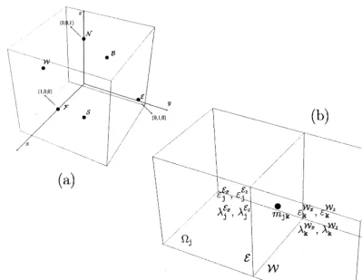
Fig. 3. a Scheme of the division of the domain V among processors. b Flow of information among processors, the shaded areas

Ž .

Fig. 4. A 2-D slice of Model 1 at ys0. The anomaly measures 2 km in the y direction.

Ž

multiple ones to be read by each processor Newman

.

and Alumbaugh, 1997 . In Fig. 3a, the planes

repre-sent the virtual boundaries created by assigning a portion of the domain V to each processor. Natu-rally, it is possible to do this assignment in different ways, we chose the displayed one. The processor number 1 solves the DDFE only in R , and simulta-11

neously, the other processors perform their calcula-tions in their respective regions.

The time needed to get the solution is usually longer than one-fourth of the time with a serial code

Ž

on one processor assuming that processors of the

.

same kind are used . This happens because on each iteration level ‘adjacent’ processors must interchange information, so that step 2 of the proposed algorithm

Ž

is adequately performed: In Fig. 3b a slice of Fig.

.

3a for constant y , the shaded regions of R12 to the right of the vertical virtual boundary and of R21

below the horizontal one involve just one column and one row, respectively of cells neighbour to subdomains in R . Therefore, all the coefficients11

´a, n

and ln

associated with the aforementioned row and column must be sent to processor number 1 in order to build the corresponding right-hand side

Table 2

Performance on the IBM SP_r2 for the presented models w x

CPU time s

Processors 1 4 8 16

Model 1, YX-mode, 10 Hz 1867.2 338.71 164.96 78.96

y3

Model 2, YX-mode, 10 Hz 6948.71 1370.94 632.87 329.05

tors bn_{. Clearly, the same is valid for the other three}

regions; the interchange of information among pro-cessors is simultaneously done at the end of step 2. We asserted that the DDFE is naturally paralleliz-able not only because of the description given above, but also due to the fact that the amount of data to be transferred is not large. As sketched in Fig. 3b, the shaded region lies on only a single subdomain width. It is easily seen that the flow of information grows with the number of processors. Therefore, the effi-ciency of the algorithm reaches its peak for some number of them, and beyond that number, it be-comes useless to employ more. However, for the

Ž .

number of processors available 16 , we did not experience this situation in our calculations.

4. Synthetic examples

We present results of two models suggested in the

Ž .

COMMEMI project Zhdanov et al., 1997 . The first

Ž .

one Model 1 is displayed in Fig. 4; it consists of a conductive block of 2 Srm embedded in a homoge-neous Earth with conductivity 0.01 Srm. The anomaly measures 1=2=2 km. We set the dimen-sions of our computational domain to be 16=16= 12 km; an air layer measuring 1 km in height and with conductivity s0_s10y7 Srm was included. The absorbing boundary condition employed makes it unnecessary to use a thicker air layer; this asser-tion is supported by performed numerical tests.

A 58=64=32-element inhomogeneous grid was used for this model, the smallest elements were of course located within and around the inhomogeneity. Two frequencies were considered: 10 Hz to test the algorithm in the presence of strongly damped fields, and 0.1 Hz to check if the numerical procedure can cope with the stationary component of the solution; this case is also useful to study the boundary condi-tion behaviour.

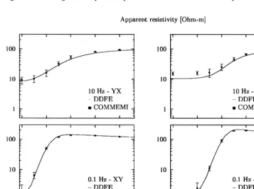
To test our algorithm, we show two principal apparent resistivities, rx y and ry x, corresponding to

Ž . Ž . Ž .

polarizations Es E,0,0 , Hs 0, H,0 XY-mode

Ž . Ž . Ž .

and Es 0, E,0 , Hs H,0,0 YX-mode ,

respec-tively. The results of the above-mentioned work are presented as error bars; taking as mid-points the means of the data after rejecting outliers, the bars measure 2d₁, twice the standard deviation of the reduced data set.

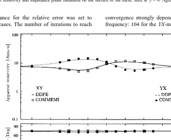
Fig. 7. Apparent resistivity and impedance phase measured on the surface of the earth, slice at ys0. Agreement between both results is very good.

The tolerance for the relative error was set to 10y4

in all cases. The number of iterations to reach

convergence strongly depends on the mode and the frequency: 104 for the YX-mode at 10 Hz, to 457 for

the same mode at 0.1 Hz. The results obtained are, in general, in very good agreement with those of the referenced paper, as can be seen in Fig. 5. The two graphs situated on the left side of the figure show measurements along the x-axis for y_s0; the two graphs on the right side display measurements made along the y-axis for xs0. Finally, in Table 2, we display the performance of our algorithm on an SP2 parallel supercomputer at Purdue University. The results correspond to the YX-mode at 10 Hz.

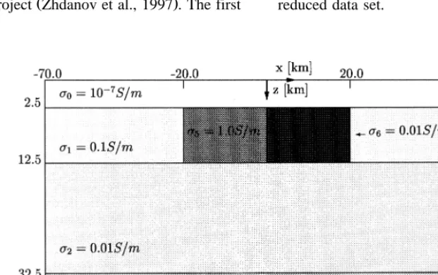
Ž .

The second model we solved Model 2 is shown in Fig. 6. It consists of two blocks of 20=40=10 km with conductivities s_s1.0 Srm and s_s0.01 Srm immersed in a three-layered earth with depths of 10, 20, and 27.5 km. The upper layer, where the blocks lie, has conductivity s_s0.1 Srm, i.e., the two blocks are chosen to be conductive and resistive, respectively, compared to their host. For the second and third layers, the conductivity values were chosen to be s_s0.01 and 10.0 Srm, respectively. The air layer thickness is 2.5 km, therefore, the domain as a whole comprises 140=120=60 km. As in the for-mer case, we chose s_s10y7 _S

rm for the air layer conductivity.

Contrary to Model 1 for which many results obtained with different methods were submitted, for Model 2 just one author sent data — obtained with an integral method. We have already mentioned

Ž

other existing solutions for this model Mackie et al.,

.

1993 , but we are not aware of any solution provided by FE methods.

The results we show in Figs. 7 and 8 — 2D slices for ys0 and 30 km, respectively — were obtained with an inhomogeneous grid of 54=54=32 ele-ments, and relative error tolerance of 10y4 at a frequency of 10y3 Hz.

5. Conclusions

We have presented an iterative finite element method for solving the forward three-dimensional magnetotelluric problem. The method has many

in-Ž .

teresting features, among them we can mention a the nonconforming finite element basis chosen that allows us to write the unknowns corresponding to

the magnetic field in terms of the ones of the electric field; and minimizes the amount of information

Ž .

transferred among processors; b the domain de-composition approach that makes it possible to work with small matrices, minimizing storage and memory

Ž .

requirements; c the absorbing boundary conditions introduced proved to perform very well, making it possible to work with relatively small computational

Ž .

domains without introducing inaccuracies; d the method is naturally parallellizable, therefore making the solution of large and complicated models possi-ble.

Acknowledgements

The authors wish to thank the SuperComputing Center of Purdue University, and the RHRK, Univer-sity of Kaiserslautern, for providing CPU time and technical advice. This work was financially sup-ported by the Agencia Nacional de Promocion

´

Cientıfica

´

y Tecnologica

´

under contract BID-802_rOC-AR. Many thanks to Peter Weidelft and Phil Wannamaker for reviews.

Appendix A

Here we show the final form of the 12=12 linear system to be solved in each of the subdomains in which we divide the domain V. Throughout this appendix we assume we have nxPnyPnz subdo-mains; and to clearly state the algebraic problem associated with the iterative procedure, it is more convenient to number the subdomains V_j and all variables with three indices rst. Therefore, the sub-domains neighbouring to V_{r s t} are those with one subscript increased or decreased by one.

We will also change the notation for the coeffi-cients defined on the faces Gr s t. For example, for the

Ž .

Ž .

in Eq. 10a by the basis functions in the order given in Table 1, and replacing the coefficients for the

magnetic field in term of the ones of the electric

Ž .

field obtained from Eq. 10b .

°

c11 c12 c13 c14 c15 c16 0 0 0 0 0 0

¶

c₂₂ c₂₃ c₂₄ c₂₅ c₂₆ 0 0 0 0 0 0

c33 c34 0 0 0 0 0 0 c3 11 c3 12

c₄₄ 0 0 0 0 0 0 c_{4 11} c_{4 12} c55 c56 0 0 c59 c5 10 0 0

c66 0 0 c69 c6 10 0 0 Cs

c₇₇ c₇₈ c₇₉ c_{7 10} c_{7 11} c_{7 12} c88 c89 c8 10 c8 11 c8 12

c₉₉ c_{9 10} 0 0

c10 10 0 0

c11 11 c11 12

¢

c12 12

ß

where

781 1 1036 h hx y

c₁₁s h h h_{x y z}s_{r s tq}

ž

ž

5040 ivm 784 hz

h h_{x z} h h_{x z WW}

q

/

q

/

qh h 1x z

Ž

yds1

.

br s t

h_y h_y

q

Ž

1yi

.

ds1h h ax z r s t,

y59 1 1036 h hx y

c₁₂s h h h_{x y z}s_{r s tq}

ž

ž

5040 ivm 784 hz

h hx z h hx z

q

/

y

/

,

hy hy

269 1 1036 h hx y

c₁₃s h h h_{x y z}s_{r s ty}

ž

5040 ivm 784 hz

h hx z

q

/

,

hy

c₁₄sc ,₁₃

1

c15sy h ,z

ivm

1

c₁₆s h ,_z ivm

781 1 1036 h h_{x y}

c22s h h hx y zsr s tq

ž

ž

5040 ivm 784 h_z

h hx z h hx z EE

q q qh h 1_{x z}

Ž

yd_{s n}

.

b_{r s t}

y

/

/

hy hy

q

Ž

1yi

.

ds nyh h ax z r s t,

c23sc ,13

c24sc ,14

c25sc ,16

c26sc ,15

781 1 1036 h hx y

c₃₃s h h h_{x y z}s_{r s tq}

ž

ž

5040 ivm 784 hz

h h_{x z} h h_{x y SS}

q

/

q

/

qh hx y

Ž

1_ydt1

.

br s t

h_y h_z

q

Ž

1yi

.

dt1h h ax y r s t,

y59 1 1036 h h_{x y}

c₃₄s h h h_{x y z}s_{r s tq}

ž

ž

5040 ivm 784 h_z

h hx z h hx y

q

/

y

/

,

y59 1 1036 h hx y the indices r, s, and t, respectively; this was not explicitly written for the sake of simplicity. The Kronecker deltas in the definition of the c s arei j

included to write in the same expression terms con-tributing either on G, the border of the domain V, or inside it. The coefficient ar s t that appears in the

Ž .

former, according to its definition below, Eq. 4 , has

Ž .1r2

the form ar s ts sr s t_r2vm .

We mentioned above that b is a complex itera-tion parameter defined on the rectangles building

Gr s t with a positive real part and a negative

imagi-nary part, which is a requirement for the algorithm to

guarantee uniqueness of the solution and for the

Ž .

iterative algorithm to converge Douglas et al., 2000 . We defined b to be an average of the values of the coefficients ar s t on both sides of any given interface

Ž . Ž .

times 1yi . With this choice Eq. 12 resembles

Ž .

the absorbing boundary condition 6 for the interior boundaries. It is still an open question if another choice for b can diminish the number of iterations for the algorithm to converge.

Finally, the 12-element vector building the right-hand side of the linear system of equations, at the

nq1 iteration level has the following form:

°

WW EE_x, n EEn

The contribution of the source term must of course be added to the vector bn _{. If an XY-polarization is}

r s t

Ž .

assumed the quantity — 1r4 h h hx y zsr s t E zp m — where zm is the mid-point of Vr s ty is added to the first, second, third, and fourth elements. In the case of a YX-polarization, the contribution goes to the fifth, sixth, ninth, and tenth elements.

References

Alumbaugh, D.L., Prevost, G.A., Shadid, J.N., 1996. Three-di-mensional wide band electromagnetic modeling on massively parallel computers. Radio Sci. 31, 1–23.

element methods: implementation, postprocessing and error estimates. R.A.I.R.O. Modelisation, Mathematique et Analyses´ ´

Numerique 9, 7–32.´

Douglas, J. Jr., Paes-Leme, P.J., Roberts, J.E., Wang, J., 1993. A parallel iterative procedure applicable to the approximate solu-tion of second order partial differential equasolu-tions by mixed finite element methods. Numer. Math. 65, 95–108.

Douglas, J. Jr., Hurtado, F., Pereira, F., 1997. On the numerical simulation of waterflooding of heterogeneous petroleum reser-voirs. Comput. Geosci. 1, 155–190.

Douglas, J. Jr., Santos, J., Sheen, D., 2000. A nonconforming mixed finite element method for Maxwell’s equations. Math. Model Methods Appl. Sci., In press.

Mackie, R.L., Madden, T.H., Wannamaker, P.E., 1993. Three-di-mensional magnetotelluric modeling using difference equa-tions—Theory and comparison to integral equation solutions.

Ž .

Geophysics 58 2 , 215–226.

Martinec, Z., 1997. Spectral-finite-element approach to two-di-mensional electromagnetic induction in a spherical earth. Geo-phys. J. Int. 130, 583–594.

Mogi, T., 1996. Three-dimensional modeling of magnetotelluric data using finite element method. J. Appl. Geophys. 35, 185–189.

Nedelec, J.C., 1980. Mixed finite elements in R3_{. Numer. Math.}

35, 315–341.

Nedelec, J.C., 1982. Elements finis mixtes incompressibles pour l’´

equation de Stokes dans R3_{. Numer. Math. 39, 97–112.}

´

Newman, G., Alumbaugh, D., 1997. Three-dimensional massively

parallel electromagnetic inversion: I. Theory. Geophys. J. Int. 128, 345–354.

Pacheco, P.S., 1997. Parallel Programming with MPI. Morgan Kaufmann.

Santos, J.E., Sheen, D., 1998. Global and parallelizable domain decomposed mixed FEM for 3D electromagnetic modelling.

Ž .

Comp. Appl. Math. 17 3 , 265–282.

Sheen, D., 1997. Approximation of electromagnetic fields: Part I. Continuous problems. SIAM J. Appl. Math. 57, 1716–1736. Wannamaker, P.E., Stodt, J.A., Rijo, L., 1987. A stable finite

element solution for two-dimensional magnetotelluric mod-elling. Geophys. J. R. Astron. Soc. 88, 277–296.

Wannamaker, P.E., 1991. Advances in 3D magnetotelluric mod-elling using integral equations. Geophysics 56, 1716–1728. Xiong, Z., 1992. Electromagnetic modeling of 3-D structures by

the method system iteration using integral equations.

Geo-Ž .

physics 57 12 , 1556–1561.

Zhdanov, M., Fang, S., 1996. Quasi-linear approximation in 3-D

Ž .

electromagnetic modeling. Geophysics 61 3 , 646–665. Zhdanov, M.S., Varentsov, I.M., Weaver, J.T., Golubev, N.G.,

Krylov, V.A., 1997. Methods for modelling electromagnetic fields: results from COMMEMI — the international project on the comparison of modelling methods for electromagnetic induction. J. Appl. Geophys. 37, 133–271.

Zyserman, F.I., Guarracino, L., Santos, J.E., 1999. A hybridized mixed finite element domain decomposed method for two dimensional magnetotelluric modelling. Earth, Planets Space

Ž .