Özlem Terzi, Eda Çevik 10
SDU International Journal of Technological Science Vol. 4, No 1, June 2012
pp. 10-19
RAINFALL ESTIMATION USING ARTIFICIAL NEURAL NETWORK
METHOD
Özlem Terzi∗, Eda Çevik
Abstract
In this study, artificial neural network (ANN) models were developed to estimate monthly total rainfall (RMT) for
Isparta. The rainfall data from Senirkent, Uluborlu, Eğirdir, Yalvaç and Isparta stations in Isparta, operated by the Turkish State Meteorological Service were used to estimate RMT. Also, multiple linear regression (MLR)
models were developed using the same input parameters for rainfall estimation. The results of ANN and MLR models were compared with measured rainfall values to evaluate performance of the developed models. The comparisons showed that there was a good agreement between the ANN estimations and measured rainfall values.
Key Words: Rainfall, Artificial Neural Networks, Multi Linear Regression, Isparta
YAPAY SİNİR AĞLARI METODU İLE YAĞIŞ TAHMİNİ
Özet
Bu çalışmada, Isparta’nın aylık toplam yağış değerlerini (RMT) tahmin temek için yapay sinir ağı (YSA)
modelleri geliştirilmiştir. RMT’yi tahmin etmek için Devlet Meteoroloji İşleri Genel Müdürlüğü’nden alınan
Senirkent, Uluborlu, Eğirdir, Yalvaç ve Isparta istasyonlarına ait yağış verileri kullanılmıştır. Aynı zamanda, aynı girdi parametreleri kullanılarak çoklu lineer regresyon (ÇLR) modelleri geliştirilmiştir. Geliştirilen modellerin performanslarını değerlendirmek için ölçülmüş yağış değerleri ile YSA ve ÇLR modelleri karşılaştırılmıştır. Karşılaştırmalar YSA tahminleri ile ölçülmüş yağış değerleri arasında iyi bir uyuşma olduğunu göstermiştir.
Anahtar Kelimeler: Yağış, Yapay Sinir Ağları, Çoklu Lineer Regresyon, Isparta
1. INTRODUCTION
The rainfall constitutes the available water resources on land and is vital for human. Short-term extreme rainfall leads to flood while long time no rainfall occurred is cause the drought. Therefore, rainfall is an important parameter in determining of water budget, drought analysis and planning of water resources. The latest developments in artificial intelligence provide an alternative approach to estimate rainfall.
Many researchers have investigated the applicability of artificial neural networks (ANN) to problems in the hydrological and meteorological areas such as solar radiation (Dorvlo et al., 2002; Mohandes et al., 2000), river flow (Imrie et al., 2000; Dibike and Solomatine, 2001; Kumar et al., 2004), short-term stream flow (Zealand et al., 1999), rainfall-runoff (Braddock et al., 1998; Tokar and Johnson, 1999; Lin and Chen, 2004), evaporation (Keskin and Terzi,
2006; Sudheer et al., 2002; Andersen and Jobson, 1982), wind speed (Mohandes et al., 1998) and rainfall estimation (French et al., 1992; Tapidor et al., 2004; Chiang et al., 2007; Lin and Wu, 2009; Çevik, 2009). Bodri and Cermak (1999) developed an ANN model for precipitation forecasting. They trained back-propagation neural networks with actual monthly precipitation data from two Moravian meteorological stations for a time period of 38 years. The predicted amounts are next-month-precipitation and summer precipitation in the next year. They showed that the ANN models provided a good fit with the actual data and a high applicability in prediction of extreme precipitation. Luk et al. (2000) adopted ANNs to forecast short-term rainfall for an urban catchment. They trained ANNs to recognize historical rainfall patterns as recorded from a number of gauges in catchment for reproduction of relevant patterns for new rainstorm events. They investigated the effect of temporal and spatial information on short-term rainfall forecasting. They found that the ANNs provided the accurate predictions and that the network with lower lag consistently produced better performance. Ramirez et al. (2005) is used ANN technique to construct a nonlinear mapping between output data from a regional ETA model and surface rainfall data for the region of São Paulo State, Brazil. They evaluated a methodology for rainfall forecasting in São Paulo State using ANN and numerical weather prediction model outputs. In order to analyze the ANN performance, they also developed a multiple linear regression (MLR) model. The results show that the ANN model has a better performance than an MLR model. Hung et al. (2009), developed real time ANN based rainfall forecasting model using observed rainfall records in both space and time. They applied the developed ANN model to derive rainfall forecast from 1 to 6 h ahead at 75 rain gauge stations in the study area as forecast point from the data of three consecutive years (1997–1999). They showed that results were highly satisfactory for rainfall forecast 1 to 3 h ahead. Sensitivity analysis indicated that the most important input parameter beside rainfall itself is the wet bulb temperature in forecasting rainfall. Based on these results, they recommended that the developed ANN model can be used for real-time rainfall forecasting and flood management in Bangkok, Thailand.
The objective of the study is to develop rainfall estimation model for Isparta station using artificial neural networks (ANN) method; to compare the ANN models to multiple linear regression (MLR) models; and to evaluate the potential of ANN for estimating rainfall.
2. ARTIFICIAL NEURAL NETWORKS
Neural networks are composed of simple elements operating in parallel. These elements are inspired by biological nervous systems. As in nature, the network function is determined largely by the connections between elements. A neural network can be trained to perform a particular function by adjusting the values of the connections (weights) between the elements. Commonly neural networks are adjusted, or trained, so that a particular input leads to a specific target output. Such a situation is shown in Figure 1. Here, the network is adjusted, based on a comparison of the output and the target, until the sum of square differences between the target and output values becomes the minimum. Typically, many such input/target output pairs are used to train a network. Batch training of a network proceeds by making weight and bias changes based on an entire set (batch) of input vectors. Incremental training changes the weights and biases of a network as needed after presentation of each individual input vector. Neural networks have been trained to perform complex functions in various fields of application including pattern recognition, identification, classification, speech, vision, and control systems (Demuth and Beale, 2001).
Figure 1. Basic principle of artificial neural networks
Feed forward ANNs comprise a system of neurons, which are arranged in layers. Between the input and output layers, there may be one or more hidden layers. The neurons in each layer are connected to the neurons in a subsequent layer by a weight w, which may be adjusted during training. A data pattern comprising the values xi presented at the input layer i is
propagated forward through the network towards the first hidden layer j. Each hidden neuron receives the weighted outputs wijxijfrom the neurons in the previous layer. These are summed
to produce a net value, which is then transformed to an output value upon the application of an activation function (Imrie et al., 2000). A typical three-layer feed-forward ANN is shown in Figure 2.
Figure 2. A typical three-layer feed-forward ANN
In Figure 2, a typical ANN consists of three layers, namely input, hidden and output layers. Input layer neurons are x1, x2… xn; hidden layer neurons are h1, h2… hm; and output layer neurons are o1, o2… ok.
A neuron consists of multiple inputs and a single output. The sum of the inputs and their weights lead to a summation operation as,
θ + =
∑
= n i ij ij j w x NET 1 (1)in which wij is established weight, xij is input value, θ is bias that additional inputs with
unitary connection weights and NETj is input to a node in layer j. Neural Network including connections (called weights) between neurons Compare Adjust weights Input Output Target x1 x2 xn h1 h2 hm o1 o2 ok w w Output Layer Hidden Layer Input Layer
The output of a neuron is decided by an activation function. There are a number of activation functions that can be used in ANNs such as step, sigmoid, threshold, linear etc. The sigmoid activation function, f(x), commonly used, can be formulated mathematically as:
[
1 exp( )]
/ 1 ) (x x f = + − (2)[
1 exp( )]
/ 1 ) ( j j j f NET NET OUTPUT = = + − (3)The back-propagation learning algorithm is one of the most important historical developments in neural networks. This learning algorithm is applied to multilayer feed-forward networks consisting of processing elements with continuous and differentiable activation functions. Such networks associated with the propagation learning algorithm are also called back-propagation networks. Given a training set of input-output pairs, the algorithm provides a procedure for changing the weights in a back-propagation network to classify the given input patterns correctly. The basis for this weight update algorithm is simply the gradient-descent method as used for simple perceptrons with differentiable neurons.
For a given input-output pair, the back-propagation algorithm performs two phases of data flow. First, the input pattern is propagated from the input layer to the output layer and, as a result of this forward flow it produces an output pattern with minimum sum of square differences between output and target data. Then the error signals resulting from the difference between output pattern and an actual output are back-propagated from the output layer to the previous layers for them to update their weights (Lin and Lee, 1995).
3. THE STUDY REGION AND DATA
The Isparta city is located in the Lakes Region located in the north of the Mediterranean Region. The Isparta is between 30 º 20 'and 31 º 33' east longitudes and 37 º 18 'and 38 º 30' north latitudes. The altitude of Isparta having a surface area of 8933 km2 is the average of 1050 m. The average annual total rainfall of Isparta is 440.3 kg/m2. The most of rainfall (72.69%) is occurred winter and spring months. The summer and autumn months are quite dry (29.31% of total rainfall). While it is observed usually rain, occasional snow in winter in the study region it is observed in the form of rainstorm the in spring and summer months. The study region and the locations of rain gauges are shown in Figure 3.
Figure 3. Locations of rain gauges in Isparta
The rainfall data used to develop the ANN model are obtained from Turkish State Meteorological Service. The meteorological stations in study area are Senirkent, Uluborlu, Eğirdir, Yalvaç and Isparta stations. The data used to develop ANN model includes monthly total rainfall (RMT) observations between 1964 and 2005 years.
Figure 4 shows the average monthly rainfall taken over a period from 1964 to 2005 in Isparta. There are two peaks of rainfall in January and December months. The average annual rainfall is 5283.8 mm with the highest average monthly rainfall of approximately 859.8 mm observed in December, and the lowest average monthly rainfall of about 105.7 mm occurring in August.
Figure 4.Average monthly rainfall in Isparta
4. APPLICATION
The relationships between rainfall data of Isparta station and them of other stations (Senirkent, Uluborlu, Eğirdir and Yalvaç) were investigated first using statistical analyses. The effective variables on Isparta station are arranged in the order of Senirkent, Uluborlu, Eğirdir and Yalvaç stations according to degree of effectiveness. Artificial neural networks (ANN) models with 2, 3 and 4 inputs were developed according to the statistical analyses results. For example, model with two inputs included rainfall data of Senirkent, Uluborlu stations whereas model with three inputs consists of rainfall data of Senirkent, Uluborlu and Eğirdir stations. In this paper, ANN(i,j,k) indicates a network architecture with i, j and k neurons in input, hidden and output layers, respectively. Herein, i runs from 2, 3 to 4; j assume values of 2, 3, 4, 5, 6, 7, 8, 9 and 10 whereas k = 1 is adopted in order to decide about the best ANN model alternative.
Prior to execution of the model, standardization is done according to the following expression such that all data values fall between 0 and 1.
) X X /( ) X X (
X= i − min max− min (4)
where X is the standardized value of the Xi; Xmax and Xminare the maximum and minimum
values in all observation sequence (Sudheer et al., 2002).
The learning rate and momentum are the parameters that affect the speed of the convergence of the back-propagation algorithm. Stopping criteria is employed 10000 epochs for training. A learning rate of 0.001 and momentum 0.1 are fixed for selected network after training and model selection is completed for years 1964-1996. The trained networks are used to run a set of test data for years 1997-2005.
The adequacy of the ANN models is evaluated by considering the coefficient of determination (R2) defined, based on the rainfall estimation errors, as:
( ) ( )
(
)
( )(
)
∑
∑
= = − − − = n i i n i i i R R R R R 1 2 mean measured 1 2 model measured 2 1 (5)where n is the number of measured rainfall data, Ri(measured) and Ri(model) are monthly total rainfall (RMT) measurement and model estimations, respectively, and Rmean is the mean RMT. The root mean square error (RMSE) is used to decide the best model and defined as:
( ) ( )
(
)
∑
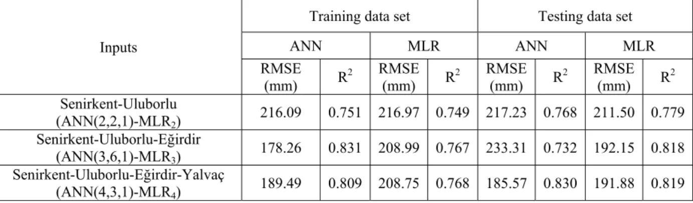
= − = n i el i measured i R R n RMSE 1 2 mod 1 (6)Also, multiple linear regression (MLR) models are developed to estimate RMT for the same input and output variables used in ANN models. The results of statistical analyses for ANN and MLR models are given in Table 1. As seen from Table 1, R2 values of ANN(2,2,1), ANN(3,6,1) and ANN(4,3,1) models are 0.768, 0.732 and 0.830 for testing set, respectively. Considering ANN models, ANN(4,3,1) model has the best R2 and the lowest RMSE values. In Table 1, comparing the performance of MLR models, MLR4 have the best R2 and RMSE values for training and testing sets. The ANN(4,3,1) model with four input parameters have the higher R2 and lower RMSE values than MLR models for training and testing data set. Considering models with two and three inputs, MLR models showed better performance than ANN models. Since the coefficients of determination of ANN(4,3,1) and MLR4 models are close to each other, it can be observed that they have more or less the same performance. Also, comparing these two models, it is shown that the ANN(4,3,1) model has a lower RMSE value than the MLR4 model. Hence the ANN(4,3,1) model is selected for monthly rainfall estimation in the study region. The performance of the ANN(4,3,1) model suggests that the rainfall could be estimated easily from available rainfall data using ANN approach. This result is of significance in situation where a hydrological model is to be developed with limited data.
Table 1. The coefficient of determination (R2) and root mean square error (RMSE) of ANN and MLR models
Inputs
Training data set Testing data set
ANN MLR ANN MLR
RMSE
(mm) R2 RMSE (mm) R2 RMSE (mm) R2 RMSE (mm) R2 Senirkent-Uluborlu (ANN(2,2,1)-MLR2) 216.09 0.751 216.97 0.749 217.23 0.768 211.50 0.779 Senirkent-Uluborlu-Eğirdir (ANN(3,6,1)-MLR3) 178.26 0.831 208.99 0.767 233.31 0.732 192.15 0.818 Senirkent-Uluborlu-Eğirdir-Yalvaç (ANN(4,3,1)-MLR4) 189.49 0.809 208.75 0.768 185.57 0.830 191.88 0.819
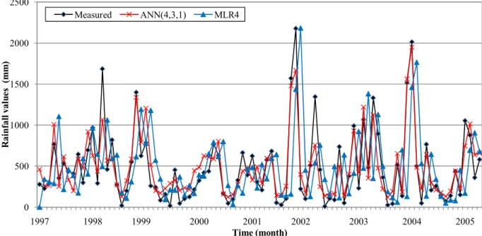
In order to expose the performance of ANN(4,3,1) model, results of the ANN(4,3,1) and MLR4 models are plotted versus rainfall values in Figure 5. The ANN(4,3,1) and MLR4 model comparison plot is around 45° straight line which implies that there are no bias effects. The results of ANN(4,3,1) and MLR4 model and RMT values are presented in Figure 6. Figure 6 shows a good agreement between the developed models and measurements of rainfall values.
Figure 5. Comparison rainfall values with ANN(4,3,1) and MLR4 models for testing data set 0 500 1000 1500 2000 2500 1997 1998 1999 2000 2001 2002 2003 2004 2005 R ai nfa ll v al ue s (m m ) Time (month) Measured ANN(4,3,1) MLR4
Figure 6. Modeled and measured rainfall values for testing data set
The measured and estimated average monthly rainfall values and the relative percentage errors are presented in Table 2 for training and testing data sets. As shown in Table 2, the relative percentage errors range from -5.89 to 0.14 %.
Table 2. Average monthly rainfall values and relative percentage errors
Models
Training data set Testing data set Average monthly rainfall
E* (%) Average monthly rainfall E* (%) Measured Estimated Measured Estimated
ANN(2,2,1) 474.78 478.46 -0.77 489.81 501.41 -2.34 ANN(3,6,1) 474.78 474.12 0.14 489.81 518.66 -5.89 ANN(4,3,1) 474.78 476.85 -0.44 489.81 505.12 -3.13 MLR2 474.78 474.85 -0.01 489.81 499.80 -2.04 MLR3 474.78 475.33 -0.12 489.81 503.68 -2.83 MLR4 474.78 475.20 -0.09 489.81 503.45 -2.78
5. CONCLUSIONS
The estimating of rainfall is of great importance in terms of water resources management, human life and their environment. It can be met with the incorrect or incomplete estimation problems because rainfall estimation is affected from the geographical and regional changes and properties. Also, because the current rainfall models in the literature are specific to the region, they are not directly used and are needed to adapt for study region. For this reason, the various rainfall estimation models have been developed to estimate rainfall for Isparta in this study. The developed ANN and MLR models with various inputs are compared to measured rainfall values. In all analyses, ANN model with four inputs have higher R2 (0.830) and lower RMSE values (185.57) for testing data set. It is shown that the ANN(4,3,1) model are superior among ANN models. Comparing the performance of the ANN(4,3,1) and MLR4 models, it can be observed that they are performed in a more similar way. The MLR models with two and three inputs show better performance than ANN models with these inputs. The performance of the ANN(4,3,1) model suggests that the rainfall could be estimated easily from available rainfall data using ANN approach. Finally, ANN models can be used for estimating rainfall in which measurement system has failed or to estimate missing rainfall data in hydrological modeling studies.
Acknowledgement This research was supported by the SDU Unit of Scientific Research
Projects, Project no. 1440-YL-06.
REFERENCES
Andersen ME, Jobson HE (1982). Comparison of techniques for estimating annual lake evaporation using climatological data. Water Resour. Res. 18:630-636.
Bodri L, Cermak V (1999). Prediction of Extreme Precipitation using a Neural Network: Application to Summer Flood Occurence in Moravia. Adv. Eng. Soft. 31:311-321.
Braddock RD, Kremmer ML, Sanzogni L (1998). Feed-forward artificial neural network model for forecasting rainfall-runoff. Environmetrics. 9:419–432.
Chiang Y-M, Chang F-J, Jou B J-D, Lin P-F (2007). Dynamic ANN for precipitation estimation and forecasting from radar observations. J. Hydrol. 334:250–261.
Çevik E (2009). Rainfall forecasting with artificial neural networks method. M.Sc. Thesis, Suleyman Demirel University Graduate School of Natural and Applied Sciences, Isparta Turkey, p.51, (In Turkish).
Demuth H, Beale M (2001). Neural network toolbox user’ guide—version 4.
Dibike YB, Solomatine DP (2001). River flow forecasting using artificial neural networks. Phys. Chem. Earth (B) 26:1-7.
Dorvlo ASS, Jervase, JA, Al-Lawati A (2002). Solar radiation estimation using artificial neural networks. Appl. Energy. 71:307-319.
French MN, Krajewski W-F, Cuykendall RR (1992). Rainfall forecasting in space and time using a neural network. J. Hydrol. 137(1-4):1-31.
Hung NQ, Babel MS, Weesakul S, Tripathi NK (2009). An artificial neural network model for rainfall forecasting in Bangkok, Thailand. Hydrol. Earth Syst. Sci. 13:1413–1425. Imrie CE, Durucan S, Korre A (2000). River flow prediction using artificial neural networks:
generalization beyond the calibration range. J. Hydrol. 233:138-153.
Keskin ME, Terzi Ö (2006). Artificial neural network models of daily pan evaporation. J. Hydrol. Eng. 11(1):65-70.
Lin G-F, Chen L-H (2004). A non-linear rainfall-runoff model using radial basis function network. J. Hydrol. 289:1–8.
Lin CT, Lee CSG (1995). Neural fuzzy systems, Prentice Hall P T R 797, New Jersey.
Lin G-F, Wu M-C (2009). A hybrid neural network model for typhoon-rainfall forecasting. J. Hydrol. 375:450–458.
Luk KC, Ball JE, Sharma A (2000). A study of optimal model lag and spatial inputs to artificial neural network for rainfall forecasting. J. Hydrol. 227:56-65.
Mohandes M, Rehman S, Halawani TO (1998). A neural networks approach for wind speed prediction. Renew. Energy. 13:345-354.
Mohandes M, Balghonaim A, Kassas M, Rehman S, Halawani TO (2000). Use of radial basis functions for estimating monthly mean daily solar radiation. Solar Energy. 68:161-168. Ramirez MCV, Velhob HFC, Ferreira NJ (2005). Artificial neural network technique for
rainfall forecasting applied to the Sa˜o Paulo region. J. Hydrol. 301:146–162.
Sudheer KP, Gosain AK, Mohana Rangan D, Saheb SM (2002). Modelling evaporation using an artificial neural network algorithm. Hydrolog. Proces. 16:3189-3202.
Tapiador FJ, Kidd C, Hsu K-L, Marzano F (2004). Neural networks in satellite rainfall estimation. Meteorol. Appl. 11:83–91.
Tokar AS, Johnson PA (1999). Rainfall-runoff modeling using artificial neural networks. J. Hydraul. Eng. 4:232-239.
Zealand CM, Burn DH, Simonovic SP (1999). Short term streamflow forecasting using artificial neural networks. J. Hydrol. 214:32-48.