Arbitrage Asymmetry and the Idiosyncratic
Volatility Puzzle
ROBERT F. STAMBAUGH, JIANFENG YU, and YU YUAN∗
ABSTRACT
Buying is easier than shorting for many equity investors. Combining this arbitrage asymmetry with the arbitrage risk represented by idiosyncratic volatility (IVOL) ex-plains the negative relation between IVOL and average return. The IVOL-return relation is negative among overpriced stocks but positive among underpriced stocks, with mispricing determined by combining 11 return anomalies. Consistent with arbi-trage asymmetry, the negative relation among overpriced stocks is stronger, especially for stocks less easily shorted, so the overall IVOL-return relation is negative. Further supporting our explanation, high investor sentiment weakens the positive relation among underpriced stocks and, especially, strengthens the negative relation among overpriced stocks.
DOES A STOCK’S EXPECTEDreturn depend on “idiosyncratic” volatility that does not arise from systematic risk factors? This question has been investigated empirically since virtually the inception of classical asset pricing theory. Earlier empirical investigations often find no relation, consistent with classical theory, or find a positive relation between expected return and idiosyncratic volatility (IVOL).1Recent empirical research on this topic, beginning notably with Ang et al. (2006), instead tends to find a negative relation between expected return
∗Stambaugh is with the Wharton School of the University of Pennsylvania and NBER, Yu is
with the Carlson School of Management at the University of Minnesota and the PBC School of Finance at Tsinghua University, and Yuan is with the Shanghai Advanced Institute of Finance at Shanghai Jiao Tong University and the Wharton Financial Institutions Center at the University of Pennsylvania. We are grateful for helpful comments from Robert Hodrick, Xiaoji Lin, ˇLuboˇs P ´astor, Zhe Zhang, two anonymous referees, an Associate Editor, seminar participants at Carnegie Mellon University, the Federal Reserve Bank of Dallas, Georgetown University, HKUST, Michigan State University, Peking University, SAC Capital Advisors, Shanghai Advanced Institute of Finance, Singapore Management University, Southwest University of Finance and Economics, University of Calgary, University of Miami, University of Minnesota, University of Oxford, University of Pennsylvania, University of Southern California, University of Texas at Dallas, and University of Toronto, and conference participants at the 2013 China International Conference in Finance, the 2013 SFS Cavalcade, the 2013 SIFR Conference on Rethinking Beta, the 2013 NBER Fall Asset Pricing Meeting, the 2013 Jacobs Levy Equity Management Center Conference, and the 2014 FMRC Conference on New Frontiers in Finance. We also thank Edmund Lee and especially Jianan Liu for excellent research assistance.
1The classic study finding no relation between expected return and IVOL is Fama and MacBeth (1973), who acknowledge the methodological issues raised by Miller and Scholes (1972) in their reexamination of Douglas (1968). A more recent study finding no relation is Bali and Cakici (2008).
DOI: 10.1111/jofi.12286
and IVOL. As Ang et al. discuss, earlier studies reporting a positive IVOL effect either do not examine IVOL at the individual stock level or do not sort directly on IVOL. The negative relation appears to be robust to various specification concerns raised by recent studies (Chen et al. (2012)). While a positive relation is accommodated by various theoretical departures from the classical paradigm, the negative relation has presented more of a puzzle.2
This study presents an explanation for the observed negative relation be-tween IVOL and expected return. We start with the principle that IVOL rep-resents risk that deters arbitrage and the resulting reduction of mispricing. In keeping with previous literature, we refer to risk that deters arbitrage as arbi-trage risk.3We then combine this familiar concept with what we term arbitrage asymmetry: many investors who would buy a stock they see as underpriced are reluctant or unable to short a stock they see as overpriced.4
Combining the effects of arbitrage risk and arbitrage asymmetry implies the observed negative relation between IVOL and expected return. To see this, first note that stocks with greater IVOL, and thus greater arbitrage risk, should be more susceptible to mispricing that is not eliminated by arbitrageurs. Among overpriced stocks, the IVOL effect in expected return should therefore be negative—those with the highest IVOL should be the most overpriced. Sim-ilarly, among underpriced stocks, the IVOL effect should be positive, as the highest IVOL stocks should then be the most underpriced. With arbitrage asymmetry, however, arbitrage should eliminate more underpricing than over-pricing, due to the greater amount of arbitrage capital devoted to long positions as compared to short positions. As a result, the differences in the degree of un-derpricing associated with different levels of IVOL should be smaller than the IVOL-related differences in overpricing. That is, the negative IVOL ef-fect among overpriced stocks should be stronger than the positive IVOL efef-fect among underpriced stocks. When aggregating across all stocks, the negative IVOL effect should therefore dominate and create the observed IVOL puzzle.
Arbitrage asymmetry exists at both the investor level and the stock level. Some investors are more able or willing to short than are other investors, and some stocks are more easily shorted than are other stocks. We present a simple model that incorporates both dimensions of arbitrage asymmetry. The basic mechanism, as in the above intuition, is that a given level of arbitrage risk is shared by more capital for long positions than for short positions. In
Studies finding a positive relation include Lintner (1965), Tinic and West (1986), Lehmann (1990), Malkiel and Xu (2002), and Fu (2009).
2Explanations for a positive relation are provided in, for example, Merton (1987), Barberis and Huang (2001), Malkiel and Xu (2002), and Ewens, Jones, and Rhodes-Kropf (2013).
3Studies addressing the role of arbitrage risk in mispricing include DeLong et al. (1990), Pontiff (1996), Shleifer and Vishny (1997), Mitchell, Pulvino, and Stafford (2002), and Wurgler and Zhuravskaya (2002).
addition, the model implies that, among overpriced stocks, the negative IVOL effect should be stronger for stocks that are less easily shorted.
Our explanation of the IVOL puzzle is supported by the data. A key element of our empirical work is constructing a proxy for mispricing. To do so, for each stock, we average its rankings associated with 11 return anomalies that survive adjustment for the three factors of Fama and French (1993). Sorting stocks based on this composite anomaly ranking allows us to investigate the IVOL effect for various degrees of relative mispricing within the cross-section. As predicted, the IVOL effect is significantly negative (positive) among the most overpriced (underpriced) stocks, and the negative effect among the overpriced stocks is significantly stronger. Moreover, consistent with our simple model, we find that the negative IVOL effect among overpriced stocks is stronger for stocks less easily shorted, as proxied by stocks with low institutional ownership (IO). We also find that the dependence of the IVOL effect on the direction of mispricing is robust to excluding smaller firms. At the same time, small-firm stocks also exhibit a stronger negative IVOL effect when overpriced, consistent with small-firm stocks being less easily shorted than large-firm stocks.
Additional implications of our explanation emerge when we consider varia-tion over time in the market-wide direcvaria-tion of mispricing. When overpricing is strongest, we should observe the strongest negative IVOL effect among stocks classified as relatively overpriced by the cross-sectional anomaly ranking. Sim-ilarly, when underpricing is its strongest, we should observe the strongest positive IVOL effect among stocks classified as relatively underpriced. With ar-bitrage asymmetry, this variation in IVOL effects over time should be stronger for stocks that are relatively overpriced. When aggregating across all stocks, the average negative relation between IVOL and expected return observed by previous studies should be stronger when there is a market-wide tendency for overpricing.
To identify periods in which a given mispricing direction is more likely, we use the index of market-wide investor sentiment constructed by Baker and Wurgler (2006).5Consistent with the above predictions, the negative IVOL ef-fect among overpriced stocks is significantly stronger following months when investor sentiment is high, and the positive IVOL effect among underpriced stocks is significantly stronger following months when investor sentiment is low. These inferences are further supported by evidence that a time-series regression of an IVOL return spread (high minus low) on investor senti-ment produces a significantly negative coefficient for both overpriced and un-derpriced stocks. Arbitrage asymmetry implies that this variation over time in IVOL effects should be stronger among the overpriced stocks. Consistent with this prediction, the time-series regression reveals significantly stronger
sentiment-related variation in the IVOL effect among the overpriced stocks. When aggregating across stocks, the overall negative IVOL effect on expected return should be stronger following high sentiment, and this prediction is con-firmed in our results.
The relation between IVOL and expected return has been explored exten-sively in the literature. Numerous studies consider interactions between IVOL and average anomaly returns, often viewing the latter as a reflection of mis-pricing. Several studies also explore interactions between short selling and the IVOL effect. While various empirical results in previous studies are consis-tent with our explanation of the IVOL effect, those studies include neither our explanation of the IVOL effect nor our set of empirical results that strongly support this explanation. The literature also includes alternative explanations of the IVOL puzzle that may be at work to some degree, but they are unable to explain the joint set of empirical results we present. The related literature is too extensive to review comprehensively, but as we present our evidence, we address the extent to which (i) our explanation of the IVOL puzzle is con-sistent with previous results and (ii) alternative explanations are inconcon-sistent with our results.
The remainder of the paper is organized as follows. SectionIdiscusses the joint roles of arbitrage asymmetry and arbitrage risk in allowing a stock’s mispricing to survive the forces of arbitrage. The analysis includes the simple model mentioned above, as well as a discussion of how a given level of IVOL can contribute more to the arbitrage risk of short positions than that of long positions. SectionIIdescribes our empirical measure of relative cross-sectional mispricing, based on a composite ranking that combines 11 return anomalies. Section III presents our basic cross-sectional results analyzing the effect of mispricing on the IVOL effect. We first use portfolio sorts to show that the IVOL effect is positive among underpriced stocks but is more strongly negative among overpriced stocks. We then use the cross-section of individual stocks to estimate the form of the relation between mispricing and the IVOL effect. Finally, we show that the negative IVOL effect among overpriced stocks is stronger among stocks with low IO, for which short-sale impediments are likely to be more important. SectionIVexplores the time-series implications of our setting, using investor sentiment as a proxy for the direction of market-wide tendencies toward overpricing or underpricing. Section V shows that, while the negative IVOL effect among overpriced stocks is stronger among smaller stocks, consistent with smaller stocks being shorted less easily, the dependence of the IVOL effect on mispricing is robust to eliminating smaller stocks. Section VIreviews the study’s main conclusions.
I. Arbitrage Risk and Arbitrage Asymmetry
Arbitrage risk is related to IVOL. If arbitrageurs can neutralize their expo-sure to benchmark risks, a seemingly reasonable assumption, then IVOL—as opposed to total volatility—is more closely related to arbitrage risk. Pontiff (2006), for example, provides a simple setting in which a stock’s IVOL rep-resents its arbitrage risk. He shows that the greater is a stock’s IVOL, the smaller is a mean-variance investor’s desired position size for a given level of alpha (mispricing). In other words, higher IVOL implies greater deterrence to price-correcting arbitrage.
Arbitrage asymmetry is well established. Institutions engaged in shorting, such as hedge funds, are rather small in aggregate compared to mutual funds and other institutions that do not short. Hong and Sraer (2014) place primary emphasis on this size disparity in arguing that short-sale impediments are important. They cite the low use of actual shorting by mutual funds, often due to investment policy restrictions, as documented by Almazan et al. (2004), as well as mutual funds’ low use of derivatives, as documented by Koski and Pontiff (1999). D’Avolio (2002) finds that shorting costs, while generally low, increase in the dispersion of opinion about a stock, consistent shorting becoming more expensive precisely when less optimistic investors would wish to short a stock whose price is driven up by more optimistic investors. Lamont (2012) discusses various impediments to short selling, and he also argues that impediments can become more severe when a stock becomes more overpriced, sometimes due to an action by a firm to deter shorting of its stock.
Section I.A below presents a simple model capturing the combined roles of arbitrage risk and arbitrage asymmetry. Mean-variance investors in a one-period setting are subject to arbitrage asymmetry when exploiting mispricing induced by noise traders. The basic mechanism at work is that, with arbitrage asymmetry, the amount of capital bearing a given degree of IVOL in shorting overpriced securities is less than the amount of capital bearing the same IVOL in buying underpriced securities. As a result, for a given level of IVOL, the demands of noise traders can exert a relatively greater effect on equilibrium alpha when those demands go in the direction of producing overpricing as opposed to underpricing.
Arbitrage asymmetry exists at both the investor level and the stock level. Some investors are more able or willing to short than other investors, and some stocks are more easily shorted than other stocks. Our model incorporates both investor-level and stock-level shorting impediments. To do so simply, within the modeling confines of an empirical study, we divide stocks and investors into two groups each. One group of investors is more able to short than the other, and one group of stocks is more easily shorted than the other. Specifically, the less constrained group of investors can short all stocks, while the more constrained group of investors can short only the group of stocks more easily shorted.
the positive relation among the underpriced stocks. This implication abstracts from differences among stocks in shorting impediments, in that it aggregates across the two stock groups that differ in the ease of shorting. Those stock-level differences play a role in the model as well. In particular, the negative relation between alpha and IVOL among overpriced stocks is steeper within the stocks less easily shorted than within those more easily shorted.
The simple one-period setting of the model includes arbitrage asymmetry, but arbitrage risk—IVOL—does not depend on whether a position is long or short. In that setting, what differs between long and short positions is the amount of capital that bears the arbitrage risk. In Section I.B below, we discuss how a given level of IVOL can translate into arbitrage risk that is itself asymmetric. In particular, short positions involve a greater risk of margin calls.
A. A Simple Model
Securities are held by mean-variance investors, index funds, and noise traders. The mean-variance investors have the single-period objective
max
ω
ω′µ− A 2ω
′Vω
, (1)
where µ is the vector of expected excess returns on the N risky assets, the
ith element ofω is the fraction of wealth invested in asset i, and V is the variance-covariance matrix of returns, assumed to be of the form
V =σm2ββ′+, (2)
where σm2 is the variance of the market return,β is the vector of the assets’ market betas, andis a diagonal matrix whoseith diagonal element isσǫ,2i, the idiosyncratic return variance of asseti.6The noise traders have asset demands given exogenously by theN-vectorz, andqis the fraction of the market owned by index funds. In this simplified setting, index funds are best viewed more broadly as including investors who limit deviations from a benchmark portfolio. We assume that the elements ofzandβ are uncorrelated in the cross-section, and we also assume that the market equity premium,µm, is the same as what it would be ifzwere the zero vector. Specifically,µm=Aσm2.
The mean-variance investors comprise two groups,IMandIH. GroupIMhas total stock market capitalM, which is allocated across stocks according to the vector of optimal weightsωM; these investors can short only the firstN1of the
N stocks. Investor group IH has stock-market capital H and optimal weights ωH; these investors can short allNstocks. Denote bysthe vector of the assets’ total market capitalizations. Market clearing requires
MωM+HωH =(1−q)s−z. (3)
Define the “excess” noise-trader demand for assetias
yi =(1−q)si−zi, (4)
wheresiandzi denote theith elements ofsandz.
For each asseti, this model delivers the following result forαi(=µi−βiµm) as Ngrows large with N1a constant fraction ofN: if the investors in group IM (constrained group) have a nonzero position in stocki(i.e.,ωM,i=0), then
αi =Ayi σǫ,2i
M+H, (5)
while if the investors in groupIMhave a zero position in stocki(i.e.,ωM,i =0), then
αi =Ayi σǫ,2i
H . (6)
Derivations are provided in the Appendix.
For a given level of excess noise-trader demand, yi, equations (5) and (6) reveal the effects of arbitrage asymmetry in the relation betweenαi and arbi-trage risk (σǫ,i). Among underpriced stocks with a given positiveyi, the relation betweenαiandσǫ,iis positive, whereas it is negative for overpriced stocks with a given negative yi. The positive relation for underpriced stocks is given by equation (5), in which M+H appears in the denominator. The negative re-lation among overpriced stocks is also given by equation (5) for the first N1
stocks that investor group IM (constrained group) can short. For the remain-ing overpriced stocks, the negative relation is instead given by equation (6), in which only Happears in the denominator, giving a steeper relation than in equation(5). Thus, when averaging across stocks in the groups more and less easily shorted, the negative relation betweenαi andσǫ,i for overpriced stocks is steeper than the positive relation for the underpriced stocks. This implica-tion reflects investor-level arbitrage asymmetry, in that it averages across the stock-level differences in shorting ease. The result also obtains in the special case of no such stock-level differences, that is, the case in which investors in groupIMcannot short any of the Nstocks (N1=0).
The role of stock-level arbitrage asymmetry also emerges from equations(5) and(6). Among the overpriced stocks, the negative relation betweenαiandσǫ,i for stocks in the group less easily shorted is given by the steeper relation in equation(6). In contrast, the negative relation for overpriced stocks in the more easily shorted group is given by the less steep relation in equation(5).
B. Asymmetric Arbitrage Risk
In the setting above, there is arbitrage asymmetry, but arbitrage risk does not depend on whether a position is long or short. What does differ between long and short positions is the amount of capital bearing the arbitrage risk. In addition to that source of asymmetry, however, the risks to arbitrageurs can differ for long versus short positions for a given level of volatility. One source of arbitrage risk, often termed “noise-trader” risk (e.g., Shleifer and Vishny (1997)), is that adverse price moves can require additional capital in order to maintain positions that involve shorting or leverage.7Such adverse moves can force capital-constrained investors to reduce their positions before realizing profits that would ultimately result from corrections of mispricing. Savor and Gamboa-Cavazos (2014) present empirical evidence on short positions that is consistent with this effect. They find that short sellers typically reduce their positions following adverse price moves, particularly if the short selling appears to be aimed at profiting from overpricing.
When IVOL is higher, substantial adverse price moves are more likely, but such moves can have different implications depending on whether the position is long or short. In general, shorting requires that a margin deposit be main-tained at some percentage of position size. If the price of the shorted stock rises, increasing the position size, additional margin capital can be required. A pur-chaser who does not employ leverage does not face margin calls, so in that case, the asymmetry in the effects of adverse price moves is obvious.8Asymmetry is still present even if purchases are made on margin. To see this, first note that a position’s margin ratio, which must typically be maintained above a specified maintenance level, is computed as
m= equity
position size. (7)
Now consider identically sized short and long positions that subsequently ex-perience identical adverse rates of return on their underlying securities. Given the identical absolute return magnitudes, both positions lose identical amounts of equity, so they still have identical values for the numerator in(7). The new denominators differ from each other, however. The position size decreases for the long position but increases for the short position, so the short position’sm
declines by a greater amount.
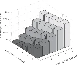
These asymmetric effects of an adverse return imply that the probability of hitting a maintenance margin level is generally more sensitive to the short leg’s IVOL than to the long leg’s IVOL. Figure1displays the probability of a long-short strategy hitting a 25% maintenance margin level within the next 12
7Engleberg, Reed, and Ringgenberg (2013) discuss additional risks of short positions, including fee increases and recalls of stock loans. Recall risk includes the possibility of occasional squeezes, as discussed, for example, by Dechow et al. (2001), who cite circumstances surrounding the stock of Amazon.com in June 1998 as a notable instance.
1 2
3 4
5 1
2 3
4 5 0
0.05 0.1 0.15 0.2
Short Leg IVOL (percent)
Long Leg IVOL (percent)
Probability of a Margin Call
Figure 1. IVOL and the probability of a margin call. The figure plots the proba-bility of a long-short strategy hitting a 25% maintenance margin level within the next 12 months when the current margin level is 35%. The current long and short positions are of equal size and have monthly IVOL values between 1% and 5%. The long (short) leg has a monthly alpha of 0.5% (−0.5%), and both legs have betas equal to one. The market portfolio’s monthly return has a mean of 0.8% and a volatility of 5%, and the monthly riskless rate is 0.3%.
months when the current margin level is 35%—a 10% cushion. The current long and short positions are of equal size and have monthly IVOL values between 1% and 5%—essentially the range for IVOLs on portfolios that we construct in SectionIII. The long (short) leg has a monthly alpha of 0.5% (−0.5%), and both legs have betas equal to one. The market portfolio’s monthly return has mean of 0.8% and standard deviation of 5%, and the monthly riskless rate is 0.3%. The asymmetric role of IVOL is evident in the plot, which reveals that the probability of a margin call is more sensitive to the IVOL of the short leg. For example, when the long-leg IVOL is 3% per month, there is nearly a fivefold increase in the margin call probability when the short-leg IVOL increases from 1% to 5%. When the long and short legs switch roles in that example, the corresponding increase in probability is less than twofold.9
II. Identifying Potential Mispricing
In our setting, mispricing is essentially the difference between the observed price and the price that would otherwise prevail in the absence of arbitrage risk and other arbitrage impediments. Of course, mispricing is not directly observable, and the best we can do is construct an imperfect proxy for it. An obvious resource for this purpose is the evidence on return anomalies, which are differences in average returns that challenge risk-based models. We construct a mispricing measure based on 11 return anomalies documented in the literature. These anomalies, used by Stambaugh, Yu, and Yuan (2012), constitute a fairly comprehensive list of those that survive adjustment for the three factors of Fama and French (1993). The 11 along with the principal studies documenting them are as follows (brief descriptions are provided in the Appendix).
1. Financial distress (Campbell, Hilscher, and Szilagyi (2008)) 2. O-Score bankruptcy probability (Ohlson (1980))
3. Net stock issues (Ritter (1991), Loughran and Ritter (1995), Fama and French (2008))
4. Composite equity issues (Daniel and Titman (2006)) 5. Total accruals (Sloan (1996))
6. Net operating assets (Hirshleifer et al. (2004)) 7. Momentum (Jegadeesh and Titman (1993)) 8. Gross profitability (Novy-Marx (2013))
9. Asset growth (Cooper, Gulen, and Schill (2008))
10. Return on assets (Fama and French (2006), Chen, Novy-Marx, and Zhang (2010))
11. Investment-to-assets (Titman, Wei, and Xie (2004), Xing (2008))
Our mispricing measure, a composite rank based on a stock’s various stock characteristics, is best interpreted as a measure of potential mispricing, pos-sibly due to noise traders, rather than as a measure of the actual mispricing that survives after arbitrage. It is possible, for instance, that a firm with a less extreme mispricing rank but high IVOL could have more mispricing that survives arbitrage than a firm with a more extreme ranking but low IVOL.
We combine the above anomalies to produce a univariate monthly measure that correlates with the degree of relative mispricing in the cross-section of stocks. While each anomaly is itself a mispricing measure, our objective in combining them is to produce a single measure that diversifies away some noise in each individual anomaly and thereby increases precision when exploring the empirical implications of our setting.
growth receive the highest rank. The higher the rank, the greater the relative degree of overpricing according to the given anomaly variable. A stock’s com-posite rank is then the arithmetic average of its ranking percentile for each of the 11 anomalies. We refer to the stocks with the highest composite ranking as the most “overpriced” and to those with the lowest ranking as the most “un-derpriced.” The mispricing measure is purely cross-sectional, so it is important to note that these designations at best denote only relative mispricing. At any given time, for example, a stock identified as the most underpriced might ac-tually be overpriced. The mispricing measure would simply suggest that this stock is the least overpriced within the cross-section. We return to this point later, when investigating the role of investor sentiment over time. Throughout the study, the stock universe each month consists of all NYSE/Amex/NASDAQ stocks with share prices greater than five dollars and for which at least five of the anomaly variables can be computed. We remove penny stocks because Chen et al. (2012) find that the IVOL effect—the puzzle we seek to explain—is es-pecially robust when those stocks are excluded. The five-anomaly requirement typically eliminates about 10% of the remaining stocks.
Evidence that our mispricing measure is effective in diversifying some of the noise in anomaly rankings can be found in the range of average returns produced by sorting on our measure. For example, in each month, we assign stocks to 10 categories based on our measure and then form a value-weighted portfolio for each decile. The following month’s spread in benchmark-adjusted returns between the two extreme deciles averages 1.48% over our sample pe-riod, August 1965–January 2011. (The returns are adjusted for exposures to the three equity benchmarks constructed by Fama and French (1993): MKT, SMB, and HML.) In comparison, if value-weighted decile portfolios are first formed for each individual anomaly ranking, and the returns on those portfolios are then combined with equal weights across the 11 anomalies, the correspond-ing spread between the extreme deciles is 0.87%. In other words, averagcorrespond-ing the anomaly rankings produces an extra 61 bps per month as compared to averaging the anomaly returns. (Thet-statistic of the difference is 4.88.)
We also find in the above comparison that ranking on our mispricing mea-sure creates additional abnormal return primarily among the stocks classified as overpriced. For example, of the 61 bps improvement in the long-short return spread reported above, 57 bps come from the most overpriced portfolio—the short leg of the corresponding arbitrage strategy—and only 4 bps come from the most underpriced—the long leg. This asymmetry in improvement in arbi-trage profits is consistent with arbiarbi-trage asymmetry: With the latter asymme-try, one expects overpricing to be greater than underpricing, so a better identi-fication of mispricing should yield greater improvement in arbitrage profits for overpriced stocks than for underpriced stocks.
III. IVOL Effects in the Cross-Section
The latter returns are computed as the residuals in a regression of each stock’s daily return on the three factors defined by Fama and French (1993): MKT, SMB, and HML. We estimate IVOL in this manner primarily to address the puzzling negative relation between IVOL and expected return found by Ang et al. (2006) and confirmed by a number of subsequent studies using the same approach. There are alternative approaches to estimating IVOL, such as the EGARCH model in Fu (2009) based on monthly returns, but the simple es-timate used here performs relatively well as a measure of forward-looking IVOL. Indeed, in a comparison of a number of IVOL estimation methods in terms of their cross-sectional rank correlations with realized daily IVOL in the subsequent month, Jin (2013) finds that past realized volatility, as used here, outperforms GARCH and EGARCH estimates and performs similarly to estimates from a simple autoregressive model.
In this section, we investigate the role of mispricing in the cross-sectional relation between alpha and IVOL. Section III.A presents the results based on portfolio sorts, an approach robust to the functional form of the relation between the IVOL effect and mispricing. We then estimate this functional form in Section III.B, using the cross-section of individual stocks. The role of stock-level arbitrage asymmetry is explored in Section III.C, using IO as a proxy for shorting impediments.
A. Mispricing and IVOL Effects
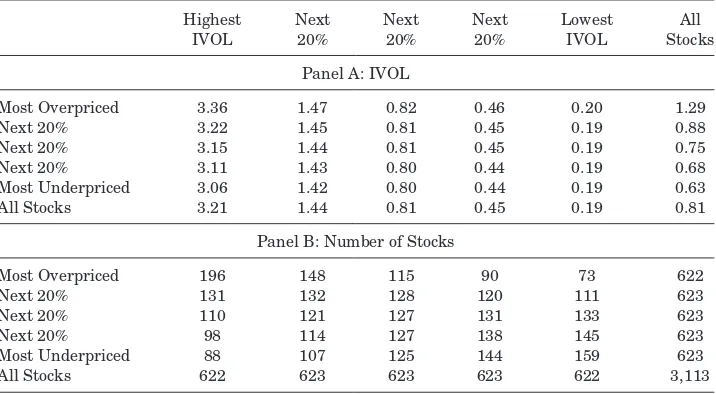
Each month, portfolios are constructed by first sorting on individual stock IVOL, forming five categories, and then sorting independently by the mis-pricing measure, again forming five categories. We next construct 25 portfo-lios defined by the intersections of this 5×5 sort, and we value-weight the stocks’ returns when computing portfolio returns. Panel A of Table Ireports the typical individual stock IVOL within each portfolio. Note that, given the independent sorting, the range for IVOL is very similar across the different levels of mispricing. The IVOL within each mispricing level, reported in the last column, increases monotonically from the most underpriced to the most overpriced stocks. This pattern also emerges in Panel B of TableI, which re-ports the average number of stocks in each portfolio: the high-IVOL portfolio contains significantly more (less) stocks than the low-IVOL portfolio among the most overpriced (underpriced) stocks. To the extent that overpriced stocks are more likely to be shorted, a related result appears in Duan, Hu, and McLean (2010), who find that stocks with high short interest have higher IVOL.
Table I
Individual Stock IVOL and Number of Stocks in the Double-Sorted Portfolios
Panel A reports the typical individual stock IVOL within each portfolio, first computing the median IVOL each month and then averaging the medians across months. Panel B reports the average number of stocks in each portfolio. The 25 portfolios are formed by independently sorting on IVOL and the mispricing measure. The latter is the average of the ranking percentiles produced by 11 anomaly variables. We compute IVOL, following Ang et al. (2006), as the standard deviation of the most recent month’s daily benchmark-adjusted returns, with the latter equal to the residuals in a regression of each stock’s daily return on the three factors defined by Fama and French (1993): MKT, SMB, and HML. The sample period is from August 1965 to January 2011.
Highest Next Next Next Lowest All
IVOL 20% 20% 20% IVOL Stocks
Panel A: IVOL
Most Overpriced 3.36 1.47 0.82 0.46 0.20 1.29
Next 20% 3.22 1.45 0.81 0.45 0.19 0.88
Next 20% 3.15 1.44 0.81 0.45 0.19 0.75
Next 20% 3.11 1.43 0.80 0.44 0.19 0.68
Most Underpriced 3.06 1.42 0.80 0.44 0.19 0.63
All Stocks 3.21 1.44 0.81 0.45 0.19 0.81
Panel B: Number of Stocks
Most Overpriced 196 148 115 90 73 622
Next 20% 131 132 128 120 111 623
Next 20% 110 121 127 131 133 623
Next 20% 98 114 127 138 145 623
Most Underpriced 88 107 125 144 159 623
All Stocks 622 623 623 623 622 3,113
impediments imply that high-volatility stocks are more likely to be overpriced than underpriced as a result of excessive optimism or pessimism—sentiment— of noise traders. Of course, nonsentiment components of noise-trader demand, such as those reflecting slow recognition of information relevant even to stocks easier to value, can contribute to mispricing at all levels of volatility. Our expla-nation of the IVOL puzzle is neither supported nor refuted by volatility-related components of noise-trader demand; the model presented earlier treats such demand (denoted byz) as exogenous.
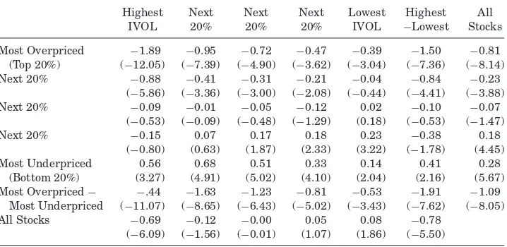
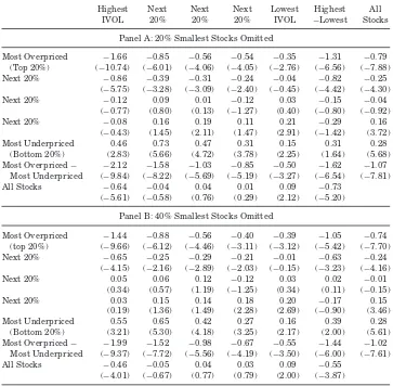
Table II, which contains the first set of our main results, reports average benchmark-adjusted monthly returns for each of the 25 portfolios. We see evidence consistent with the role of IVOL-driven arbitrage risk in mispricing. Among the stocks most likely to be mispriced, as identified by our mispricing measure, we expect to see the magnitude of mispricing increase with IVOL. The patterns in average returns are consistent with this prediction. For the most overpriced stocks, the average returns are negative and monotonically
Table II
Idiosyncratic Volatility Effects in Underpriced versus Overpriced Stocks
This table reports average benchmark-adjusted returns for portfolios formed by sorting stocks independently on IVOL and the mispricing measure. The mispricing measure is the average of the ranking percentiles produced by 11 anomaly variables. Also reported are results based on sorting by IVOL within the entire stock universe. Benchmark-adjusted returns are calculated asain the regression
Ri,t=a+bMKTt+cSMBt+dH MLt+ǫi,t,
where Ri,t is the excess percent return in montht. The sample period is from August 1965 to January 2011. Allt-statistics (in parentheses) are based on the heteroskedasticity-consistent stan-dard errors of White (1980).
Highest Next Next Next Lowest Highest All IVOL 20% 20% 20% IVOL −Lowest Stocks
Most Overpriced −1.89 −0.95 −0.72 −0.47 −0.39 −1.50 −0.81 (Top 20%) (−12.05) (−7.39) (−4.90) (−3.62) (−3.04) (−7.36) (−8.14) Next 20% −0.88 −0.41 −0.31 −0.21 −0.04 −0.84 −0.23
(−5.86) (−3.36) (−3.00) (−2.08) (−0.44) (−4.41) (−3.88) Next 20% −0.09 −0.01 −0.05 −0.12 0.02 −0.10 −0.07
(−0.53) (−0.09) (−0.48) (−1.29) (0.18) (−0.53) (−1.47) Next 20% −0.15 0.07 0.17 0.18 0.23 −0.38 0.18
(−0.80) (0.63) (1.87) (2.33) (3.22) (−1.78) (4.45) Most Underpriced 0.56 0.68 0.51 0.33 0.14 0.41 0.28
(Bottom 20%) (3.27) (4.91) (5.02) (4.10) (2.04) (2.16) (5.67) Most Overpriced− −.44 −1.63 −1.23 −0.81 −0.53 −1.91 −1.09
Most Underpriced (−11.07) (−8.65) (−6.43) (−5.02) (−3.43) (−7.62) (−8.05) All Stocks −0.69 −0.12 −0.00 0.05 0.08 −0.78
(−6.09) (−1.56) (−0.01) (1.07) (1.86) (−5.50)
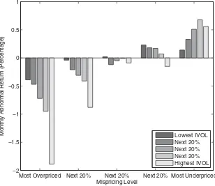
portfolios equal to −1.50% per month (t-statistic: −7.36).10 For the most un-derpriced stocks, the average returns are positive and generallyincreasingin IVOL, with the difference between the highest and lowest IVOL portfolios equal to 0.41% per month (t-statistic: 2.16). For the stocks in the middle of the mis-pricing scale, there is no apparent IVOL pattern, and the highest-versus-lowest difference is only−0.10% per month (t-statistic:−0.53). The role of mispricing in determining the strength and direction of IVOL effects is readily apparent in Figure2, which plots the average benchmark-adjusted returns reported in TableII.
Also, evident in Table II and Figure 2 is the asymmetry in IVOL effects predicted by arbitrage asymmetry. Recall that the IVOL break points are the
Most Overpriced Next 20% Next 20% Next 20% Most Underpriced −2
−1.5 −1 −0.5 0 0.5 1
Mispricing Level
Monthly Abnormal Return (Percentage) Lowest IVOL Next 20% Next 20% Next 20% Highest IVOL
Figure 2. Monthly abnormal returns of portfolios ranked by mispricing level and IVOL. The figure plots the average monthly abnormal return on portfolios formed in a 5×5 sort that ranks independently by mispricing level and IVOL. Abnormal returns are calculated by adjusting for exposures to the three Fama-French (1993) factors. The average ranking percentile of 11 anomalies is used to measure the relative level of mispricing. The sample period covers August 1965–January 2011.
same across the mispricing quintiles in Table II and that the ranges of av-erage IVOLs are therefore very similar across the mispricing quintiles. As a result, we can see that the negative IVOL effect among the overpriced stocks is stronger than the positive IVOL effect among the underpriced stocks. The negative highest-versus-lowest difference among the most overpriced stocks is 3.7 times the magnitude of the corresponding positive difference among the most underpriced stocks.
Given the asymmetry in the strengths of the negative and positive IVOL effects among ovepriced and underpriced stocks, aggregating across all stocks results in the negative overall IVOL effect reported in the last row of TableII. Among all stocks, consistent with the IVOL puzzle observed in the literature, average return is monotonically decreasing in IVOL, with the highest-versus-lowest difference equal to−0.78% per month (t-statistic:−5.50).
who argue that IVOL proxies for a return-reversal effect, Han and Lesmond (2011), who argue that the IVOL effect is due to market microstructure biases, and Bali and Cakici (2008), who argue that equal-weighted portfolios do not show a robust negative IVOL effect. Chen et al. find that the results in support of these three studies are not robust to excluding penny stocks and microcaps.11 Other studies reporting a negative relation include Jiang, Xu, and Yao (2009) and Guo and Savickas (2010). As Ang et al. (2006) discuss, the earlier studies finding a positive IVOL effect either do not examine IVOL at the individual stock level or do not sort on IVOL directly. A more recent study by Fu (2009) finds a positive IVOL effect, rather than a negative one, but Guo, Kassa, and Ferguson (2014) and Fink, Fink, and He (2012) argue that the positive rela-tion between expected return and IVOL found in Fu (2009) is due to the use of contemporaneous information in the conditional variance model, and that the positive relation does not survive after controlling for such information. Rachwalski and Wen (2013) find that expected return is negatively related to recent IVOL but positively related to less recent IVOL. Similarly, Cao and Xu (2010) find that expected return is negatively related to short-run IVOL but positively related to long-run IVOL. Short-run volatility, in the months imme-diately following the identification of mispricing, seems especially relevant to arbitrageurs, and in that regard our explanation applies to the negative short-run relation—our explanation does not imply a positive long-short-run relation.
The switch from a negative to a positive IVOL effect when moving from overpriced stocks to underpriced stocks is previously reported by Cao and Han (2014). Those authors also explore the role of IVOL-related arbitrage risk in mispricing by sorting stocks based on a composite of anomaly rankings, and they similarly find a significantly negative (positive) IVOL effect among the relatively overpriced (underpriced) stocks. Their results do not display sub-stantial asymmetry in the strength of those IVOL effects, nor do they discuss asymmetry or the IVOL puzzle. A potential reason asymmetry does not emerge as a feature of their study is that their anomaly ranking measure could contain less information about mispricing, as it combines only four anomalies instead of our 11, and two of those four are size and book-to-market, for which a mis-pricing interpretation must contend with a significant literature, arguing that those variables proxy instead for risk. Studies by Boehme et al. (2009) and Duan, Hu, and McLean (2010) find a strong negative IVOL effect among stocks with high shorting activity, but among stocks with low shorting activity, the negative relation becomes flatter, or even weakly positive in the case of the first study. Such a result is consistent with our explanation if shorting activity is higher among overpriced stocks.
An additional implication of our setting is that the degree of mispricing, es-pecially overpricing, should be greater among high-IVOL stocks than among
low-IVOL stocks. We also see support for this implication. The difference in average portfolio returns between the most overpriced stocks and the most un-derpriced stocks is negative and decreasing in IVOL, as shown in the next to last row in TableII. The difference between that short-long difference for the highest IVOL portfolios versus the lowest IVOL portfolios is−1.91% per month (t-statistic: −7.62). These results are consistent with Jin (2013), who finds that long-short spreads on each of 10 anomalies are more profitable among high-IVOL stocks than among low-IVOL stocks, and that this difference in profitability is attributable primarily to the short legs of each strategy. To our knowledge, Jin’s study is unique in noting this consistent asymmetry in the short legs versus the long legs across many anomaly spreads, but numerous other studies find that various return anomalies are stronger among high-IVOL stocks. Such anomalies include those based on closed-end fund discounts (Pontiff (1996)), index inclusions (Wurgler and Zhuravskaya (2002)), postearn-ings announcement drift (Mendenhall (2004)), the value premium (Ali, Hwang, and Trombley (2003)), momentum (Zhang (2006)), accruals (Mashruwala, Rajgopal, and Shevlin (2006), Pincus, Rajgopal, and Venkatachalam (2007), Li and Sullivan (2011)), “Siamese twin” stocks (Scruggs (2007)), insider trades and share repurchases (Ben-David and Roulstone (2010)), long-term reversal (McLean (2010)), asset growth (Li and Sullivan (2011), Lipson, Mortal, and Schill (2011)), Li and Zhang (2010), Lam and Wei (2011)), equity issuance (Larrain and Varas (2013)), investment to assets (Li and Zhang (2010)), and return on assets (Wang and Yu (2010)).
An alternative explanation consistent with standard asset pricing theory is that the IVOL effect reflects compensation for an omitted systematic risk factor. Barinov (2013) and Chen and Petkova (2012) conclude that IVOL proxies for sensitivity to a priced volatility factor, but this explanation also has a problem accommodating the switch in sign of the IVOL effect. If IVOL is correlated in the cross-section with the sensitivity to a systematic factor, and that factor has a negative premium, then such a scenario is consistent with the negative IVOL effect among overpriced stocks but not with the positive relation among underpriced stocks. Indeed, as we report in the Internet Appendix, if we use our 25 portfolios to estimate the sensitivities to correlation and average-variance factors, as defined in Chen and Petkova (2012), the second-stage cross-sectional regressions produce coefficient estimates with opposite signs to what Chen and Petkova obtain.
A more general factor-based scenario is that alphas are proportional to sensi-tivities to a missing risk factor. Positive alphas would then be positively related in the cross-section to the return variance attributable to the missing factor, and negative alphas would exhibit a negative relation to that variance com-ponent. If the variances attributable to the missing factor are then significant portions of the variances that we identify as idiosyncratic when using just the three Fama-French (1993; FF) factors, the signs of the IVOL effects we observe would result. To explore this alternative explanation empirically, we construct a factor consisting of the long-short daily return spread between stocks in the top and bottom quintiles of our mispricing measure. Essentially by construc-tion, stocks with high (low) alphas have high (low) sensitivities to this factor. If we then compute IVOLs using a model including this factor in addition to the FF factors, the resulting IVOLs have an average rank correlation of 99.7% with the IVOLs based on just the FF factors. In other words, our IVOL rankings are virtually unchanged if we remove from IVOL the variance attributable to this alpha-based factor. While this factor does not exhaust the set of omitted factors for which sensitivities might be highly correlated with alphas, we suggest that it does reduce the plausibility of such a scenario’s explaining the IVOL effects in expected returns. In addition, the asymmetry in the strengths of the positive and negative IVOL effects we observe would still seem to present a challenge for such an alternative explanation.
As explained earlier, a stock’s mispricing measure in a given month is con-structed by equally weighting the stock’s percentile rankings for each of 11 anomalies. Equal weights across the 11 anomalies are simple and transpar-ent but not crucial for our results. We obtain results very similar to those in TableII when applying weights that are instead proportional to rolling five-year averages of the coefficients in a cross-sectional regression of monthly benchmark-adjusted returns on anomaly rankings.12 Rather than regress-ing returns on all 11 individual anomaly rankregress-ings, we first group anoma-lies into five clusters, equally weighting the rankings within each cluster.
As compared to weights produced by regressing on the individual rankings, the regression-based weights on each cluster are substantially more stable over time and are rarely negative. (Three anomalies—financial distress, O-score bankruptcy probability, and investment-to-assets—often receive negative weights in a regression on the 11 individual anomalies.) The clusters are formed using the same procedure as Ahn, Conrad, and Dittmar (2009), who combine a correlation-based distance measure with the clustering method of Ward (1963). We apply this procedure using the correlation matrix of benchmark-adjusted returns on the 11 anomalies, as reported in Stambaugh, Yu, and Yuan (2012). The results corresponding to those in Table II are included in the Internet Appendix.
B. Estimating the Role of Mispricing
Our empirical analysis thus far is based on portfolio sorts, so it requires only a monotonic relation between the IVOL effect and mispricing. Such an approach is robust to this relation’s specific form but reveals less about it as a consequence. In this subsection, we use the cross-section of individual stocks to estimate the form of the relation between the IVOL effect and mispricing.
In each montht, we estimate a cross-sectional regression of the form
rte+1,i=β0+ ft(Mt,i)σt,i+ǫt+1,i, (8)
where re
t+1,i is stock i’s excess return in month t+1 minus its FF factor ad-justment, Mt,i is the stock’s mispricing proxy (the average of its 11 anomaly ranking percentiles) in month t, andσt,i is the stock’s IVOL in month t. The values of σt,i are standardized each month by subtracting the cross-sectional mean IVOL within the month and then dividing by the month’s cross-sectional standard deviation of IVOL. We estimate ft(·) as a piecewise linear function:
ft(M)= n
k=1
I(θk−1,t≤ M< θk,t)×(ak,t+bk,tM), (9)
where
ak,t+bk,tθk,t=ak+1,t+bk+1,tθk,t, k=1, . . . ,n−1, (10)
0 10 20 30 40 50 60 70 80 90 100 −300
−250 −200 −150 −100 −50 0 50 100 150
Mispricing (avg. percentile)
IVOL Effect (basis points)
Estimated IVOL Effect 90% Lower Bound 90% Upper Bound
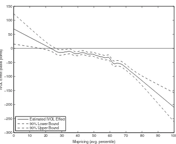
Figure 3. Estimated IVOL effects.The figure plots estimates of f(M), which is the effect of standardized IVOL on the abnormal monthly return for a stock whose mispricing ranking percentile (averaged over 11 anomalies) is equal toM. Estimates are computed using the August 1965–January 2011 sample period.
The function ft(M) in(8)characterizes the relation between the IVOL effect and mispricing. The month-by-month procedure described above yields an es-timated function ft(M) for each monthtin our sample (August 1965 through January 2011). These monthly values are then used in a procedure following the spirit of Fama and MacBeth (1973). For each value of mispricing (M) in 0.01 increments within [0, 1], we take the mean of the monthly function values as an estimate of the desired function, f(M)=(1/T)Tt=1 ft(M). We estimate the standard error of f(M) using the monthly series of ft(M)s.
intermediate values. This result makes sense if differences in anomaly rank-ings percentile toward the middle of the distribution do not identify econom-ically significant differences in mispricing. It seems reasonable that, if the anomaly rankings identify potential mispricing, they would do so more suc-cessfully at the extremes of those rankings.
The estimate of f(M) obtained here explains much of the overall IVOL effect obtained when aggregating across all levels of mispricing. If, in each month, we estimate a simple cross-sectional regression ofrte+1,ionσt,iand then average the slope coefficients across all months in the sample, we obtain a value of−0.0030. This estimate is close to the value of−0.0028 obtained if the estimated values of f(M) plotted in Figure3are weighted by the cross-sectional sample density of M values. The latter density is obtained by computing the cross-sectional frequency distribution ofMt,i each month and then averaging those frequency distributions across months.
One might ask whether a cross-sectional regression can shed light on whether our explanation fully accounts for the IVOL effect. In general, such a test is not possible, in that we do not know a priori the function that relates mispricing to the IVOL effect or even the no-mispricing value forMt,iat which the IVOL effect should flip signs when moving from underpricing to overpricing. The presence of shorting impediments, and thus the resulting net tendency for overpricing, implies that the no-mispricing point should be less than 50% (closer to the underpriced end), but that is as much as our explanation delivers. Suppose our explanation fully accounts for the IVOL effect, and one regressesrte+1,i on both σt,i and the interaction term Mt,iσt,i. Then, a significantly nonzero coefficient onσt,i would simply indicate that a zero value of Mt,i does not correspond to zero mispricing. On the other hand, if each month we instead run a cross-sectional regression ofre
t+1,ion both f(Mt,i)σt,iandσt,i, the average slope on the latter is−0.00017 with a t-statistic of −0.39. One should not view the latter insignificance as failure to reject the adequacy of our explanation, however, as f(Mt,i) is fit to the data. The insignificant average slope on σt,i is better viewed as suggesting that ft(M) is typically captured reasonably well by the time-aggregated function f(M).
C. Institutional Ownership and the IVOL Effect
stock-level arbitrage asymmetry and the ability of IO to proxy for that asym-metry.13Since IO is positively correlated with firm size, we follow Nagel and compute size-adjusted IO, which is the residual in a cross-sectional regression that fits the logit of IO (in percent) as a quadratic function of the logarithm of firm size. Our data on institutional holdings come from Thomson Financial Institutional Holdings and cover the period from April 1980 to January 2011.
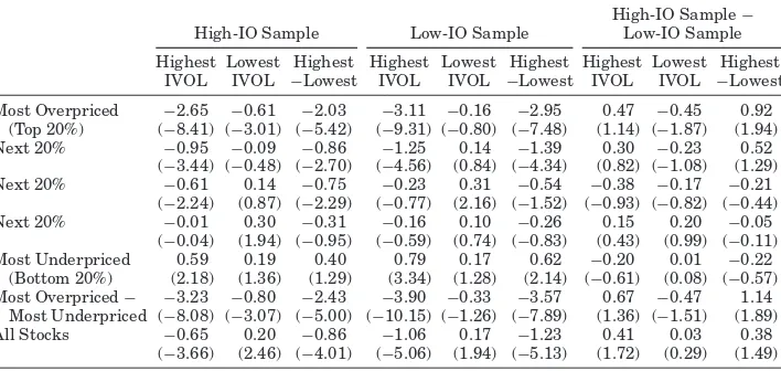
To investigate the implications of stock-level arbitrage asymmetry, we con-duct a three-way sort. First, we assign stocks to mispricing quintiles by sorting on our mispricing measure. Within each mispricing quintile, we then sort by IVOL, forming five groups, and independently by IO, forming three groups. For each mispricing quintile, TableIIIreports the average benchmark-adjusted re-turns for the “corner” portfolios of the IVOL-IO double sort. The last row reports results based on the double sort within the entire stock universe.
Within a given mispricing quintile, the independent sorting produces very similar ranges of IVOL across the different IO groupings, thereby allowing us to examine differences in the strength of the IVOL effect across different IO levels. For example, within the most overpriced stocks—those of the greatest interest in exploring the effects of stock-level arbitrage asymmetry—the high and low IVOL values for the high-IO group are 5.12% and 0.37%, while the corresponding values for the low-IO group are 5.25% and 0.33%.
Stock-level arbitrage asymmetry predicts that the negative IVOL effect among overpriced stocks should be stronger for stocks less easily shorted. This prediction is supported by the first row of TableIII, which reports results for the most overpriced stocks. Among low-IO stocks (those less easily shorted), the difference in average monthly returns between the portfolios with high and low IVOL is−2.95%, while the corresponding difference for high-IO stocks is −2.03%. This economically significant difference in IVOL effects of 92 bps per month has at-statistic of−1.94, yielding a p-value of 0.026 for a test of the zero-difference null against the one-sided alternative hypothesis implied by stock-level arbitrage asymmetry.
Stock-level arbitrage asymmetry should play less of a role in the IVOL effect among stocks that are less overpriced, and we see that pattern in Table III. Among stocks in the second highest mispricing quintile, the negative IVOL effect for low-IO stocks is again stronger than that for high-IO stocks, but the difference of 52 bps and its associated p-value of 0.099 corresponds to less economic and statistical significance than observed among the most over-priced stocks. Among the remaining three mispricing quintiles, the differences in IVOL effects between the two IO groups are relatively small and statisti-cally insignificant, consistent with the implication that stock-level arbitrage asymmetry should matter only among overpriced stocks.
Table III
Idiosyncratic Volatility Effects in Subsamples of High versus Low Institutional Ownership
This table reports average benchmark-adjusted returns for portfolios constructed by sorting inde-pendently on IVOL and IO within each quintile of the mispricing measure. The high-IO (low-IO) subsample consists of the top (bottom) 30% of stocks sorted on size-adjusted IO, computed following Nagel (2005): each quarter, we regress the logit of the IO percentage on log(size) and the square of log(size) and take the regression residual as size-adjusted IO. The data on institutional hold-ings come from the Thomson Financial Institutional Holdhold-ings database. The mispricing quintiles are determined by sorting on the average ranking percentiles produced by 11 anomaly variables. Also reported are results based on sorting by IVOL and IO within the entire stock universe. The benchmark-adjusted returns are estimates ofain the regression
Ri,t=a+bMKTt+cSMBt+dH MLt+ǫi,t,
whereRi,tis the excess percent return in montht. The sample period is from April 1980 to Jan-uary 2011. Allt-statistics (in parentheses) are based on the heteroskedasticity-consistent standard errors of White (1980).
High-IO Sample−
High-IO Sample Low-IO Sample Low-IO Sample
Highest Lowest Highest Highest Lowest Highest Highest Lowest Highest IVOL IVOL −Lowest IVOL IVOL −Lowest IVOL IVOL −Lowest
Most Overpriced −2.65 −0.61 −2.03 −3.11 −0.16 −2.95 0.47 −0.45 0.92 (Top 20%) (−8.41) (−3.01) (−5.42) (−9.31) (−0.80) (−7.48) (1.14) (−1.87) (1.94) Next 20% −0.95 −0.09 −0.86 −1.25 0.14 −1.39 0.30 −0.23 0.52
(−3.44) (−0.48) (−2.70) (−4.56) (0.84) (−4.34) (0.82) (−1.08) (1.29) Next 20% −0.61 0.14 −0.75 −0.23 0.31 −0.54 −0.38 −0.17 −0.21
(−2.24) (0.87) (−2.29) (−0.77) (2.16) (−1.52) (−0.93) (−0.82) (−0.44) Next 20% −0.01 0.30 −0.31 −0.16 0.10 −0.26 0.15 0.20 −0.05
(−0.04) (1.94) (−0.95) (−0.59) (0.74) (−0.83) (0.43) (0.99) (−0.11) Most Underpriced 0.59 0.19 0.40 0.79 0.17 0.62 −0.20 0.01 −0.22
(Bottom 20%) (2.18) (1.36) (1.29) (3.34) (1.28) (2.14) (−0.61) (0.08) (−0.57) Most Overpriced− −3.23 −0.80 −2.43 −3.90 −0.33 −3.57 0.67 −0.47 1.14
Most Underpriced (−8.08) (−3.07) (−5.00) (−10.15) (−1.26) (−7.89) (1.36) (−1.51) (1.89) All Stocks −0.65 0.20 −0.86 −1.06 0.17 −1.23 0.41 0.03 0.38
(−3.66) (2.46) (−4.01) (−5.06) (1.94) (−5.13) (1.72) (0.29) (1.49)
Nagel (2005) observes that, within the overall stock universe, the negative IVOL effect is stronger for firms with low IO. The last row of TableIIIreveals a similar result, in that the average IVOL effect among firms with low IO exceeds the average IVOL effect among firms with high IO by a difference of 0.38%, and thet-statistic of 1.49 yields a p-value of 0.068 against the one-sided alternative. Our results reveal that this IO-related difference in the IVOL effect within the overall stock universe is attributable to the overpriced stocks, as implied by stock-level arbitrage asymmetry.
IV. Time-Varying IVOL Effects
are also those times when our relatively overpriced stocks are more likely to be overpriced in absolute terms and our underpriced stocks are less likely to be underpriced in absolute terms. At such times, the negative IVOL effect among our “overpriced” stocks should be stronger, and the positive IVOL effect among our “underpriced” stocks should be weaker. In the context of equations(5)and (6), if potential mispricing in a stock occurs due to excess noise-trader demand,
yi, then systematic variation over time in the typical values ofyi across stocks should produce variation in the strength of the corresponding IVOL effects.
To investigate such time-varying IVOL effects, we need to identify varia-tion over time in the general tendency for overpricing versus underpricing in the stock market. For this purpose, we rely on the index of market-wide in-vestor sentiment constructed by Baker and Wurgler (2006; BW). Their index is constructed as the first principal component of six underlying measures of investor sentiment: the average closed-end fund discount, the number and first-day returns of IPOs, NYSE turnover, the equity share of total new issues, and the dividend premium (log difference of average market-to-book of dividend payers versus nonpayers). These authors show that their sentiment index pre-dicts returns on stocks more likely to be susceptible to mispricing, such as stocks on small or young firms, more volatile stocks, distressed stocks, and ex-treme growth stocks. Further evidence that the BW index identifies variation in mispricing is provided by Stambaugh, Yu, and Yuan (2012), who find that the index significantly predicts long-short return spreads for each of the 11 anomalies we analyze here.
Stambaugh, Yu, and Yuan (2012) also find that the ability of sentiment to pre-dict the long-short return spreads is due largely to prepre-dictability of the short-leg returns. As these authors explain, the latter result is predicted by arbitrage asymmetry in a setting in which sentiment-driven noise traders have strongly positive demand for many stocks when sentiment is high but do not have cor-respondingly negative demand when sentiment is low, due to an inability or reluctance to sell short. In the context of equations(5)and(6), this asymmetric effect of market-wide sentiment on noise trader demand is equivalent to sen-timent’s having greater effects on the lowyis that produce overpricing than on the highyis that produce underpricing. When applied to our analysis of IVOL effects, this asymmetry implies that investor sentiment should exert a greater effect on the negative IVOL effect among overpriced stocks than on the positive IVOL effect among underpriced stocks.
sentiment measure, which removes the effects of six macrovariables. We fur-ther include six additional macrovariables that previous empirical studies re-late to expected stock returns. Our results point to little or no role for macro-factors in the sentiment-related variation in the IVOL effects that we observe.
A. Investor Sentiment and IVOL Effects
To explore the sentiment-related implications discussed above, we first con-duct a sorting-based portfolio analysis, similar to that in Table II, separately for high-sentiment and low-sentiment months. We modify the sorting proce-dure somewhat due to the shift in focus from the cross-section to the time series when investigating IVOL effects. To compare IVOL effects over time for a given level of mispricing, one would ideally maintain the same volatil-ity break points across different periods. Doing so, however, confronts the fact that average IVOL levels fluctuate substantially over time (e.g., Brandt et al. (2010)). Maintaining fixed IVOL break points in the portfolio sorting is there-fore not feasible, as it results in highly unbalanced distributions of stocks in many periods, often producing portfolios with few or no stocks. Therefore, for each mispricing level, we instead set fixed percentage break points for IVOL, forming five portfolios each period with essentially equal numbers of stocks in each portfolio. In addition to presenting results using this portfolio-based analysis, we also rerun the individual-stock-based estimation in Section III.B separately in high-sentiment and low-sentiment months.
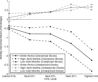
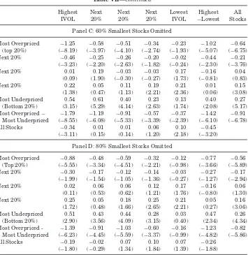
TableIVpresents the results of the portfolio-based analysis of the IVOL effect following different levels of investor sentiment. The middle three IVOL cate-gories are omitted to save space in the table. Average benchmark-adjusted re-turns for all five IVOL categories in low-sentiment and high-sentiment months are displayed in Figure4. A high-sentiment month is one in which the value of the BW sentiment index at the end of the previous month is above the median value for the August 1965–January 2011 sample period, while the low-sentiment months are those with below-median index values in the previous month.
Table IV
Idiosyncratic Volatility Effects in High-Sentiment versus Low-Sentiment Periods
This table reports average benchmark-adjusted returns for portfolios containing stocks with either the highest (top 20%) or lowest (bottom 20%) IVOL. The sort on IVOL is performed for stocks within a given range of over-/underpricing, as determined by an average of the ranking percentiles produced by 11 anomaly variables. Also reported are results based on sorting by IVOL within the entire stock universe. The benchmark-adjusted returns in high- and low-sentiment periods are estimates ofaHandaLin the regression
Ri,t=aHdH,t+aLdL,t+bMKTt+cSMBt+dH MLt+ǫi,t,
wheredH,tanddL,tare dummy variables indicating high- and low-sentiment periods, andRi,tis the excess percent return in montht. The sample period is from August 1965 to January 2011. Allt-statistics (in parentheses) are based on the heteroskedasticity-consistent standard errors of White (1980).
High-Sentiment Periods− High-Sentiment Periods Low-Sentiment Periods Low-Sentiment Periods
Highest Lowest Highest Highest Lowest Highest Highest Lowest Highest
IVOL IVOL −Lowest IVOL IVOL −Lowest IVOL IVOL −Lowest
Most Overpriced 2.84 −0.54 −2.30 −1.66 −0.36 −1.30 −1.18 −0.18 −1.00 (Top 20%) (−9.57) (−3.13) (−6.79) (−6.91) (−2.55) (−4.75) (−3.06) (−0.86) (−2.29)
Next 20% −1.24 −0.01 −1.23 −0.60 −0.16 −0.44 −0.64 0.15 −0.79
(−5.28) (−0.04) (−4.31) (−2.77) (−1.26) (−1.71) (−2.02) (0.82) (−2.07)
Next 20% −0.17 0.31 −0.48 −0.10 −0.22 0.13 −0.07 0.53 −0.60
(−0.72) (2.34) (−1.75) (−0.54) (−1.92) (0.52) (−0.25) (3.09) (−1.68)
Next 20% −0.10 0.19 −0.29 −0.04 0.11 −0.16 −0.06 0.08 −0.14
(−0.35) (1.44) (−0.84) (−0.23) (1.29) (−0.75) (−0.18) (0.49) (−0.34)
Most Underpriced 0.54 0.33 0.21 0.82 −0.12 0.94 −0.28 0.45 −0.73
(Bottom 20%) (2.43) (2.77) (0.77) (4.05) (−1.21) (4.16) (−0.93) (2.85) (−2.03) Most Overpriced− −3.38 −0.87 −2.51 −2.48 −0.24 −2.24 −0.90 −0.63 −0.27
Most Underpriced (−9.36) (−4.02) (−6.48) (−7.82) (−1.22) (−6.60) (−1.85) (−2.23) (−0.53)
All Stocks −1.06 0.26 −1.32 −0.33 −0.10 −0.23 −0.72 0.36 −1.09
(−5.75) (3.81) (−5.88) (−2.45) (−1.87) (−1.35) (−3.16) (4.16) (−3.82)
−1.30% following low sentiment—a difference of −1.00% (t-statistic:−2.29). For the most underpriced stocks, the positive IVOL effect is stronger following low sentiment than following high sentiment: among those stocks, the spread between the highest-IVOL and lowest-IVOL average returns is 0.21% follow-ing high sentiment compared to 0.94% followfollow-ing low sentiment—a difference of −0.73% (t-statistic:−2.03). These results support arbitrage asymmetry as well, in which the sentiment-related difference in IVOL effects is somewhat larger for the most overpriced stocks, although thet-statistic for the difference is modest (−0.53). When interpreting this last result, one should probably con-sider that a binary split between high- and low-sentiment periods, while useful in its simplicity, does not necessarily yield the most powerful test. Below, we estimate time-series regressions as an alternative approach.
Lowest IVOL−3 Next 20% Next 20% Next 20% Highest IVOL −2.5
−2 −1.5 −1 −0.5 0 0.5 1
IVOL Level
Monthly Abnormal Return (Percentage) Entire Period (Overpriced Stocks)High−Sent Months (Overpriced Stocks) Low−Sent Months (Overpriced Stocks) Entire Period (Underpriced Stocks) High−Sent Months (Underpriced Stocks) Low−Sent Months (Underpriced Stocks)
Figure 4. IVOL effects and investor sentiment.The figure plots the average monthly abnor-mal return on portfolios formed in a 5×5 sort that ranks first by mispricing level and then by IVOL. Results are displayed for the five portfolios in the most underpriced quintile and the five portfolios in the most overpriced quintile. Abnormal returns are calculated by adjusting for exposures to the three Fama-French (1993) factors. The average ranking percentile of 11 anomalies is used to mea-sure the relative level of mispricing. Averages are reported for the overall August 1965–January 2011 sample period as well as for high-sentiment and low-sentiment months classified using the Baker-Wurgler (2006) index.
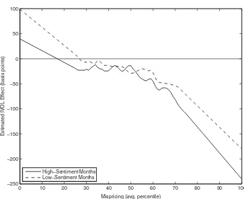
high- and low-sentiment months. Figure5displays the resulting estimates of
f(M) in the two subsamples. Consistent with the above portfolio results, the negative IVOL effect in overpriced stocks is stronger following high sentiment, and the positive IVOL effect among underpriced stocks is stronger following low sentiment. Thet-statistics for the differences between the two curves exceed −2.0 in magnitude for values of M between 20% and 30% (underpricing) as well as between 70% and 80% (overpricing). As Mtakes more extreme values at both ends, the t-statistics decline in magnitude to about −1.0, consistent with there being fewer observations in the tails and thus less precision in the estimates of f(M). We also see that sentiment exerts little if any effect on the relation between the IVOL effect andMfor intermediate values ofM, which is consistent with minimal mispricing at such values.
0 10 20 30 40 50 60 70 80 90 100 −250
−200 −150 −100 −50 0 50 100
Mispricing (avg. percentile)
Estimated IVOL Effect (basis points)
High−Sentiment Months Low−Sentiment Months
Figure 5. Estimated IVOL effects following high and low sentiment.The figure plots es-timates of f(M), which is the effect of standardized IVOL on the abnormal monthly return for a stock whose mispricing ranking percentile (averaged over 11 anomalies), is equal to M. The estimates are computed separately in high-sentiment and low-sentiment months classified using the Baker-Wurgler (2006) index for the August 1965–January 2011 sample period.
previous month. Also included as independent variables are the contemporane-ous realizations of the FF factors (MKT, SMB, and HML), so the slope onSt−1
reflects sentiment-related variation in the benchmark-adjusted returns. The dependent variable in the regressions is (i) the (excess) return on the highest IVOL portfolio, (ii) the return on the lowest IVOL portfolio, or (iii) the differ-ence between those returns. These three regressions are run separately for each mispricing category and for the overall stock universe.
The results in Table V again support our setting’s implications. Consis-tent with Table IV, the IVOL effect (highest minus lowest IVOL) is nega-tively related to investor sentiment. For the overall stock universe, the slope on St−1 is equal to −0.66 (t-statistic:−4.25), meaning that a
one-standard-deviation swing in St−1 is associated with a 66 bps difference in the IVOL
effect. In addition, the negative slope is largest in magnitude among the most overpriced stocks, and the difference between the slopes for the most overpriced versus the most underpriced stocks is equal to −0.50 (t-statistic: