The Supply and Demand for Goods

(1)

User JOEWA:Job EFF01423:6264_ch07:Pg 180:26797#/eps at 100%

26797

Wed, Feb 13, 2002 9:48 AM

7

If you have ever spoken with your grandparents about what their lives were like when they were young, most likely you learned an important lesson about economics: material standards of living have improved substantially over time for most families in most countries. This advance comes from rising in-comes, which have allowed people to consume greater quantities of goods and services.

To measure economic growth, economists use data on gross domestic prod-uct, which measures the total income of everyone in the economy. The real GDP of the United States today is more than three times its 1950 level, and real GDP per person is more than twice its 1950 level. In any given year, we can also observe large differences in the standard of living among countries. Table 7-1 shows income per person in 1999 of the world’s 12 most populous countries. The United States tops the list with an income of $31,910 per person. Nigeria has an income per person of only $770—less than 3 percent of the figure for the United States.

Our goal in this part of the book is to understand what causes these differ-ences in income over time and across countries. In Chapter 3 we identified the factors of production—capital and labor—and the production technology as the sources of the economy’s output and, thus, of its total income. Differences in in-come, then, must come from differences in capital, labor, and technology.

Our primary task is to develop a theory of economic growth called the Solow growth model. Our analysis in Chapter 3 enabled us to describe how the economy produces and uses its output at one point in time. The analysis was static—a snapshot of the economy. To explain why our national income grows, and why some economies grow faster than others, we must broaden our analysis so that it describes changes in the economy over time. By developing such a model, we make our analysis dynamic—more like a movie than a pho-tograph. The Solow growth model shows how saving, population growth, and C H A P T E R

The question of growth is nothing new but a new disguise for an age-old

issue, one which has always intrigued and preoccupied economics: the

present versus the future.

— James Tobin

180|

S E V E N

(2)

26798

Wed, Feb 13, 2002 9:48 AM technological progress affect the level of an economy’s output and its growth

over time. In this chapter we analyze the roles of saving and population growth. In the next chapter we introduce technological progress.1

7-1

The Accumulation of Capital

The Solow growth model is designed to show how growth in the capital stock, growth in the labor force, and advances in technology interact in an economy, and how they affect a nation’s total output of goods and services. We build this model in steps. Our first step is to examine how the supply and demand for goods determine the accumulation of capital. In this first step, we assume that the labor force and technology are fixed. We then relax these assumptions by intro-ducing changes in the labor force later in this chapter and by introintro-ducing changes in technology in the next.

The Supply and Demand for Goods

The supply and demand for goods played a central role in our static model of the closed economy in Chapter 3.The same is true for the Solow model. By consid-ering the supply and demand for goods, we can see what determines how much output is produced at any given time and how this output is allocated among al-ternative uses.

1_{The Solow growth model is named after economist Robert Solow and was developed in the} 1950s and 1960s. In 1987 Solow won the Nobel Prize in economics for his work in economic growth.The model was introduced in Robert M. Solow,“A Contribution to the Theory of Eco-nomic Growth,’’Quarterly Journal of Economics(February 1956): 65–94.

Income per Person Income per Person Country (in U.S. dollars) Country (in U.S. dollars)

United States $31,910 China 3,550

Japan 25,170 Indonesia 2,660

Germany 23,510 India 2,230

Mexico 8,070 Pakistan 1,860

Russia 6,990 Bangladesh 1,530

Brazil 6,840 Nigeria 770

Source: _{World Bank.}

(3)

26799

Wed, Feb 13, 2002 9:48 AM The Supply of Goods and the Production Function The supply of goods in

the Solow model is based on the now-familiar production function, which states that output depends on the capital stock and the labor force:

Y=F(K,L).

The Solow growth model assumes that the production function has constant re-turns to scale. This assumption is often considered realistic, and as we will see shortly, it helps simplify the analysis. Recall that a production function has con-stant returns to scale if

zY₌F(zK,zL)

for any positive number z.That is, if we multiply both capital and labor by z, we also multiply the amount of output by z.

Production functions with constant returns to scale allow us to analyze all quantities in the economy relative to the size of the labor force.To see that this is true, set z=1/Lin the preceding equation to obtain

Y/L₌F(K/L, 1).

This equation shows that the amount of output per worker Y/Lis a function of the amount of capital per worker K/L. (The number “1” is, of course, constant and thus can be ignored.) The assumption of constant returns to scale implies that the size of the economy—as measured by the number of workers—does not affect the relationship between output per worker and capi-tal per worker.

Because the size of the economy does not matter, it will prove convenient to denote all quantities in per-worker terms.We designate these with lowercase let-ters, so y=Y/Lis output per worker, and k=K/Lis capital per worker.We can then write the production function as

y=f(k),

where we define f(k) ₌F(k,1). Figure 7-1 illustrates this production function. The slope of this production function shows how much extra output a worker produces when given an extra unit of capital.This amount is the marginal prod-uct of capital MPK. Mathematically, we write

MPK₌f(k₊1) ₋f(k).

Note that in Figure 7-1, as the amount of capital increases, the production func-tion becomes flatter, indicating that the production function exhibits diminish-ing marginal product of capital. When k is low, the average worker has only a little capital to work with, so an extra unit of capital is very useful and produces a lot of additional output.When kis high, the average worker has a lot of capital, so an extra unit increases production only slightly.

(4)

26800

Wed, Feb 13, 2002 9:48 AM

words, output per worker y is divided between consumption per worker c and investment per worker i:

y=c+i.

This equation is the per-worker version of the national income accounts identity for an economy. Notice that it omits government purchases (which for present pur-poses we can ignore) and net exports (because we are assuming a closed economy). The Solow model assumes that each year people save a fraction sof their in-come and consume a fraction (1 −s).We can express this idea with a consump-tion funcconsump-tion with the simple form

c=(1 −s)y,

where s, the saving rate, is a number between zero and one. Keep in mind that various government policies can potentially influence a nation’s saving rate, so one of our goals is to find what saving rate is desirable. For now, however, we just take the saving rate sas given.

To see what this consumption function implies for investment, substitute (1 − s)y for cin the national income accounts identity:

y₌(1 −s)y+i.

Rearrange the terms to obtain

i=sy.

This equation shows that investment equals saving, as we first saw in Chapter 3. Thus, the rate of saving sis also the fraction of output devoted to investment.

f i g u r e 7 - 1

Output per worker, y

MPK

Capital per worker, k 1

Output, f(k)

(5)

26801

Wed, Feb 13, 2002 9:48 AM

We have now introduced the two main ingredients of the Solow model—the production function and the consumption function—which describe the econ-omy at any moment in time. For any given capital stock k, the production

func-tion y = f(k) determines how much output the economy produces, and the

saving rate sdetermines the allocation of that output between consumption and investment.

Growth in the Capital Stock and the Steady State

At any moment, the capital stock is a key determinant of the economy’s output, but the capital stock can change over time, and those changes can lead to eco-nomic growth. In particular, two forces influence the capital stock: investment and depreciation.Investment refers to the expenditure on new plant and equip-ment, and it causes the capital stock to rise.Depreciationrefers to the wearing out of old capital, and it causes the capital stock to fall. Let’s consider each of these in turn.

As we have already noted, investment per worker iequals sy. By substituting the production function for y, we can express investment per worker as a func-tion of the capital stock per worker:

i=sf(k).

This equation relates the existing stock of capital kto the accumulation of new capital i. Figure 7-2 shows this relationship. This figure illustrates how, for any value of k, the amount of output is determined by the production function f(k), and the allocation of that output between consumption and saving is determined by the saving rate s.

f i g u r e 7 - 2

Output per worker, y

y c

Investment, sf(k) Output, f(k)

i

Capital per worker, k Consumption

per worker Output

per worker

Investment per worker

(6)

26802

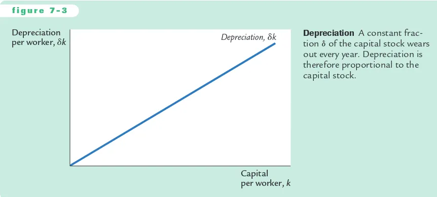
Wed, Feb 13, 2002 9:48 AM To incorporate depreciation into the model, we assume that a certain fraction

d

of the capital stock wears out each year. Here

_d

(the lowercase Greek letter delta) is called the depreciation rate. For example, if capital lasts an average of 25 years, then the depreciation rate is 4 percent per year (

_d

=0.04).The amount of

capital that depreciates each year is

_d

k. Figure 7-3 shows how the amount of de-preciation depends on the capital stock.

We can express the impact of investment and depreciation on the capital stock with this equation:

Change in Capital Stock =Investment −Depreciation

D

k = i −

d

k,

where

_D

kis the change in the capital stock between one year and the next. Be-cause investment iequals sf(k), we can write this as

D

k=sf(k) −

d

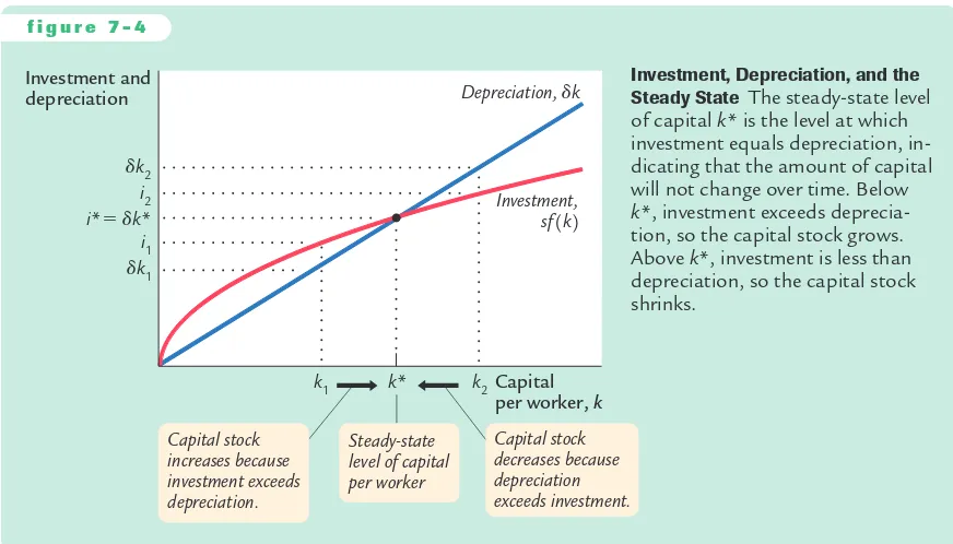
k.

Figure 7-4 graphs the terms of this equation—investment and depreciation—for different levels of the capital stock k.The higher the capital stock, the greater the amounts of output and investment.Yet the higher the capital stock, the greater also the amount of depreciation.

As Figure 7-4 shows, there is a single capital stock k*at which the amount of investment equals the amount of depreciation. If the economy ever finds itself at this level of the capital stock, the capital stock will not change because the two forces acting on it—investment and depreciation—just balance. That is, at k*,

D

k= 0, so the capital stock kand output f(k) are steady over time (rather than

growing or shrinking).We therefore call k*the steady-statelevel of capital. The steady state is significant for two reasons. As we have just seen, an omy at the steady state will stay there. In addition, and just as important, an econ-omy not at the steady state will go there.That is, regardless of the level of capital

f i g u r e 7 - 3

Depreciation

per worker, dk Depreciation, dk

Capital per worker, k

(7)

26803

Wed, Feb 13, 2002 9:48 AM

with which the economy begins, it ends up with the steady-state level of capital. In this sense,the steady state represents the long-run equilibrium of the economy.

To see why an economy always ends up at the steady state, suppose that the economy starts with less than the steady-state level of capital, such as level k1in Figure 7-4. In this case, the level of investment exceeds the amount of deprecia-tion. Over time, the capital stock will rise and will continue to rise—along with output f(k)—until it approaches the steady state k*.

Similarly, suppose that the economy starts with more than the steady-state level of capital, such as level k2. In this case, investment is less than depreciation: capital is wearing out faster than it is being replaced. The capital stock will fall, again approaching the steady-state level. Once the capital stock reaches the steady state, investment equals depreciation, and there is no pressure for the capi-tal stock to either increase or decrease.

Approaching the Steady State: A Numerical Example

Let’s use a numerical example to see how the Solow model works and how the economy approaches the steady state. For this example, we assume that the pro-duction function is2 Steady State The steady-state level of capital k* is the level at which investment equals depreciation, in-dicating that the amount of capital will not change over time. Below

k*, investment exceeds deprecia-tion, so the capital stock grows. Above k*, investment is less than depreciation, so the capital stock shrinks.

2_{If you read the appendix to Chapter 3, you will recognize this as the Cobb}_–_{Douglas production} function with the parameter

(8)

26804

Wed, Feb 13, 2002 9:48 AM

To derive the per-worker production function f(k), divide both sides of the pro-duction function by the labor force L:

= .

This equation can also be written as

y=兹k苶.

This form of the production function states that output per worker is equal to the square root of the amount of capital per worker.

To complete the example, let’s assume that 30 percent of output is saved (s= 0.3), that 10 percent of the capital stock depreciates every year (

_d

=0.1), and that the economy starts off with 4 units of capital per worker (k= 4). Given these numbers, we can now examine what happens to this economy over time.

We begin by looking at the production and allocation of output in the first year. According to the production function, the 4 units of capital per worker produce 2 units of output per worker. Because 30 percent of output is saved and invested and 70 percent is consumed,i=0.6 and c=1.4. Also, because 10 percent of the capital stock depreciates,

_d

k= 0.4.With investment of 0.6 and deprecia-tion of 0.4, the change in the capital stock is

_D

k=0.2. The second year begins with 4.2 units of capital per worker.

Table 7-2 shows how the economy progresses year by year. Every year, new capital is added and output grows. Over many years, the economy approaches a steady state with 9 units of capital per worker. In this steady state, investment of 0.9 exactly offsets depreciation of 0.9, so that the capital stock and output are no longer growing.

Following the progress of the economy for many years is one way to find the steady-state capital stock, but there is another way that requires fewer calcula-tions. Recall that

D

k=sf(k) −

d

k.

(9)

26805

Wed, Feb 13, 2002 9:48 AM

This equation provides a way of finding the steady-state level of capital per

worker,k_*_{. Substituting in the numbers and production function from our}

ex-ample, we obtain

= .

Now square both sides of this equation to find

k_*₌_9.

The steady-state capital stock is 9 units per worker.This result confirms the cal-culation of the steady state in Table 7-2.

0.3



0.1

k_*

_兹k_苶

*

Approaching the Steady State: A Numerical Example

t a b l e 7 - 2

Assumptions: y=兹k苶; s=0.3;

d

=0.1; initial k=4.0

Year k y c i

_d

k

_D

k

1 4.000 2.000 1.400 0.600 0.400 0.200

2 4.200 2.049 1.435 0.615 0.420 0.195

3 4.395 2.096 1.467 0.629 0.440 0.189

4 4.584 2.141 1.499 0.642 0.458 0.184

5 4.768 2.184 1.529 0.655 0.477 0.178

. . .

10 5.602 2.367 1.657 0.710 0.560 0.150

. . .

25 7.321 2.706 1.894 0.812 0.732 0.080

. . .

100 8.962 2.994 2.096 0.898 0.896 0.002

. . .

∞ 9.000 3.000 2.100 0.900 0.900 0.000

C A S E S T U D Y

The Miracle of Japanese and German Growth

(10)

26806

Wed, Feb 13, 2002 9:49 AM

How Saving Affects Growth

The explanation of Japanese and German growth after World War II is not quite as simple as suggested in the preceding case study. Another relevant fact is that both Japan and Germany save and invest a higher fraction of their output than the United States.To understand more fully the international differences in eco-nomic performance, we must consider the effects of different saving rates.

Consider what happens to an economy when its saving rate increases. Figure 7-5 shows such a change. The economy is assumed to begin in a steady state with saving rate s1and capital stock k*₁_{. When the saving rate increases from}_s1 _to_s2_,

the sf(k) curve shifts upward. At the initial saving rate s1 and the initial capital stock k*₁_{, the amount of investment just offsets the amount of depreciation.}

Im-mediately after the saving rate rises, investment is higher, but the capital stock and depreciation are unchanged.Therefore, investment exceeds depreciation.The capital stock will gradually rise until the economy reaches the new steady state k*₂_{, which has a higher capital stock and a higher level of output than the old}

steady state.

The Solow model shows that the saving rate is a key determinant of the steady-state capital stock.If the saving rate is high, the economy will have a large capital stock and a high level of output. If the saving rate is low, the economy will have a small capital stock and a low level of output.This conclusion sheds light on many discus-sions of fiscal policy. As we saw in Chapter 3, a government budget deficit can reduce national saving and crowd out investment. Now we can see that the long-run consequences of a reduced saving rate are a lower capital stock and lower national income. This is why many economists are critical of persistent budget deficits.

What does the Solow model say about the relationship between saving and economic growth? Higher saving leads to faster growth in the Solow model, but decades after the war, however, these two countries experienced some of the most rapid growth rates on record. Between 1948 and 1972, output per person grew at 8.2 percent per year in Japan and 5.7 percent per year in Germany, com-pared to only 2.2 percent per year in the United States.

(11)

26807

Wed, Feb 13, 2002 9:49 AM

C A S E S T U D Y

Saving and Investment Around the World

We started this chapter with an important question:Why are some countries so rich while others are mired in poverty? Our analysis has taken us a step closer to the answer. According to the Solow model, if a nation devotes a large fraction of its income to saving and investment, it will have a high steady-state capital stock and a high level of income. If a nation saves and invests only a small fraction of its income, its steady-state capital and income will be low.

Let’s now look at some data to see if this theoretical result in fact helps explain the large international variation in standards of living. Figure 7-6 is a scatterplot of data from 84 countries. (The figure includes most of the world’s economies. It excludes major oil-producing countries and countries that were communist dur-ing much of this period, because their experiences are explained by their special only temporarily. An increase in the rate of saving raises growth only until the economy reaches the new steady state. If the economy maintains a high saving rate, it will maintain a large capital stock and a high level of output, but it will not maintain a high rate of growth forever.

Now that we understand how saving affects growth, we can more fully explain the impressive economic performances of Germany and Japan after World War II. Not only were their initial capital stocks low because of the war, but their steady-state capital stocks were high because of their high saving rates. Both of these facts help explain the rapid growth of these two countries in the 1950s and 1960s.

f i g u r e 7 - 5

d_k

s₂f(k)

s₁f(k)

k₂* k₁*

Investment and depreciation

Capital per worker, k 2. . . . causing

the capital stock to grow toward a new steady state.

1. An increase in the saving rate raises investment, . . .

An Increase in the Saving Rate An increase in the saving rate simplies that the amount of investment for any given capital stock is higher. It therefore shifts the saving function upward. At the initial steady state k1*,

(12)

26808

Wed, Feb 13, 2002 9:49 AM

circumstances.) The data show a positive relationship between the fraction of output devoted to investment and the level of income per person.That is, coun-tries with high rates of investment, such as the United States and Japan, usually have high incomes, whereas countries with low rates of investment, such as Uganda and Chad, have low incomes. Thus, the data are consistent with the Solow model’s prediction that the investment rate is a key determinant of whether a country is rich or poor.

The strong correlation shown in this figure is an important fact, but it raises as many questions as it resolves. One might naturally ask, why do rates of saving and investment vary so much from country to country? There are many potential an-swers, such as tax policy, retirement patterns, the development of financial mar-kets, and cultural differences. In addition, political stability may play a role: not surprisingly, rates of saving and investment tend to be low in countries with fre-quent wars, revolutions, and coups. Saving and investment also tend to be low in countries with poor political institutions, as measured by estimates of official cor-ruption. A final interpretation of the evidence in Figure 7-6 is reverse causation:

f i g u r e 7 - 6

Investment as percentage of output (average 1960 –1992)

20 25 30 35 40

International Evidence on Investment Rates and Income per Person This scat-terplot shows the experience of 84 countries, each represented by a single point. The horizontal axis shows the country’s rate of investment, and the vertical axis shows the country’s income per person. High investment is associated with high income per person, as the Solow model predicts.

(13)

26809

Wed, Feb 13, 2002 9:49 AM

7-2

The Golden Rule Level of Capital

So far, we have used the Solow model to examine how an economy’s rate of saving and investment determines its steady-state levels of capital and income.This analy-sis might lead you to think that higher saving is always a good thing, for it always leads to greater income. Yet suppose a nation had a saving rate of 100 percent. That would lead to the largest possible capital stock and the largest possible income. But if all of this income is saved and none is ever consumed, what good is it?

This section uses the Solow model to discuss what amount of capital accumu-lation is optimal from the standpoint of economic well-being. In the next chap-ter, we discuss how government policies influence a nation’s saving rate. But first, in this section, we present the theory behind these policy decisions.

Comparing Steady States

To keep our analysis simple, let’s assume that a policymaker can set the economy’s saving rate at any level. By setting the saving rate, the policymaker determines the economy’s steady state.What steady state should the policymaker choose?

When choosing a steady state, the policymaker’s goal is to maximize the well-being of the individuals who make up the society. Individuals themselves do not care about the amount of capital in the economy, or even the amount of output. They care about the amount of goods and services they can consume. Thus, a benevolent policymaker would want to choose the steady state with the highest level of consumption.The steady-state value of k_{that maximizes consumption is}

called the Golden Rule level of capitaland is denoted k_*_gold_.3

How can we tell whether an economy is at the Golden Rule level? To answer this question, we must first determine steady-state consumption per worker. Then we can see which steady state provides the most consumption.

perhaps high levels of income somehow foster high rates of saving and invest-ment. Unfortunately, there is no consensus among economists about which of the many possible explanations is most important.

The association between investment rates and income per person is strong, and it is an important clue as to why some countries are rich and others poor, but it is not the whole story. The correlation between these two variables is far from perfect. Mexico and Zimbabwe, for instance, have had similar investment rates, but income per person is more than three times higher in Mexico. There must be other determinants of living standards beyond saving and investment. We therefore return to the international differences later in the chapter to see what other variables enter the picture.

3

(14)

26810

Wed, Feb 13, 2002 9:49 AM

To find steady-state consumption per worker, we begin with the national

in-come accounts identity

y₌c₊i

and rearrange it as

c₌y₋i.

Consumption is simply output minus investment. Because we want to find

steady-state consumption, we substitute steady-state values for output and invest-ment. Steady-state output per worker is f(k*), where k*is the steady-state capital stock per worker. Furthermore, because the capital stock is not changing in the steady state, investment is equal to depreciation

_d

k*. Substituting f(k*) for yand

d

k*for i, we can write steady-state consumption per worker as

c*₌f(k*) −

_d

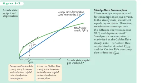
k*.

According to this equation, steady-state consumption is what’s left of steady-state output after paying for steady-state depreciation. This equation shows that an in-crease in steady-state capital has two opposing effects on steady-state consumption. On the one hand, more capital means more output. On the other hand, more cap-ital also means that more output must be used to replace capcap-ital that is wearing out. Figure 7-7 graphs steady-state output and steady-state depreciation as a func-tion of the steady-state capital stock. Steady-state consumpfunc-tion is the gap between

f i g u r e 7 - 7

Below the Golden Rule steady state, increases in steady-state capital raise steady-state consumption.

Above the Golden Rule steady state, increases The economy’s output is used for consumption or investment. In the steady state, investment equals depreciation. Therefore, steady-state consumption is the difference between output f(k*) and depreciation

_d

k*. Steady-state consumption is maximized at the Golden Rule steady state. The Golden Rule capital stock is denoted k*gold,

(15)

26811

Wed, Feb 13, 2002 9:49 AM output and depreciation. This figure shows that there is one level of the capital

stock—the Golden Rule level k*gold—that maximizes consumption.

When comparing steady states, we must keep in mind that higher levels of capital affect both output and depreciation. If the capital stock is below the Golden Rule level, an increase in the capital stock raises output more than de-preciation, so that consumption rises. In this case, the production function is steeper than the

_d

k* line, so the gap between these two curves—which equals consumption—grows as k* rises. By contrast, if the capital stock is above the Golden Rule level, an increase in the capital stock reduces consumption, since the increase in output is smaller than the increase in depreciation. In this case, the production function is flatter than the

_d

k*line, so the gap between the curves— consumption—shrinks as k* rises. At the Golden Rule level of capital, the pro-duction function and the

_d

k*line have the same slope, and consumption is at its greatest level.

We can now derive a simple condition that characterizes the Golden Rule level of capital. Recall that the slope of the production function is the marginal product of capital MPK.The slope of the

_d

k* line is

_d

. Because these two slopes are equal at k*gold, the Golden Rule is described by the equation

MPK=

_d

.

At the Golden Rule level of capital, the marginal product of capital equals the depreciation rate.

To make the point somewhat differently, suppose that the economy starts at some steady-state capital stock k* and that the policymaker is considering increasing the capital stock to k* ₊ 1. The amount of extra output from this increase in capital would be f(k*₊ 1) − f(k*), which is the marginal product of capital MPK. The amount of extra depreciation from having 1 more unit of capital is the depreciation rate

_d

. Thus, the net effect of this extra unit of capital on consumption is MPK−

_d

. If MPK−

_d

> 0, then increases in capi-tal increase consumption, so k* must be below the Golden Rule level. If MPK−

_d

< 0, then increases in capital decrease consumption, so k* must be above the Golden Rule level.Therefore, the following condition describes the Golden Rule:

MPK−

_d

=0.

At the Golden Rule level of capital, the marginal product of capital net of depre-ciation (MPK−

_d

) equals zero. As we will see, a policymaker can use this condi-tion to find the Golden Rule capital stock for an economy.4

Keep in mind that the economy does not automatically gravitate toward the Golden Rule steady state. If we want any particular steady-state capital stock, such as the Golden Rule, we need a particular saving rate to support it. Figure 7-8

4

Mathematical note: Another way to derive the condition for the Golden Rule uses a bit of cal-culus. Recall that c* = f(k*) −

_d

k*. To find the k* that maximizes c*, differentiate to find

(16)

26812

Wed, Feb 13, 2002 9:49 AM

shows the steady state if the saving rate is set to produce the Golden Rule level of capital. If the saving rate is higher than the one used in this figure, the steady-state capital stock will be too high. If the saving rate is lower, the steady-steady-state capital stock will be too low. In either case, steady-state consumption will be lower than it is at the Golden Rule steady state.

Finding the Golden Rule Steady State:

A Numerical Example

Consider the decision of a policymaker choosing a steady state in the following economy. The production function is the same as in our earlier example:

y=兹k苶.

Output per worker is the square root of capital per worker. Depreciation

_d

is again 10 percent of capital. This time, the policymaker chooses the saving rate s and thus the economy’s steady state.

To see the outcomes available to the policymaker, recall that the following equation holds in the steady state:

= s.

d

k*

 f(k*) f i g u r e 7 - 8

1. To reach the Golden Rule steady state . . .

2. . . .the economy needs the right saving rate.

Steady-state output, depreciation, and

investment per worker d_k* f(k*)

sgoldf(k*)

c*_gold

i*_gold

k*_gold Steady-state capital per worker, k_*

The Saving Rate and the Golden Rule There is only one saving rate that produces the Golden Rule level of capital k*gold. Any change in the saving rate would shift the sf(k)

(17)

26813

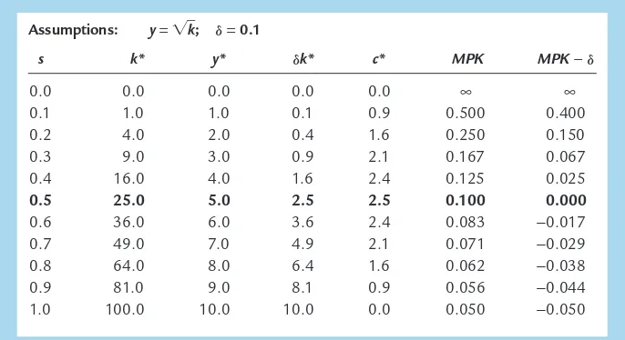
Wed, Feb 13, 2002 9:49 AM

Finding the Golden Rule Steady State: A Numerical Example t a b l e 7 - 3

Assumptions: y=兹k苶;

d

=0.1

s k* y*

_d

k* c* MPK MPK−

d

0.0 0.0 0.0 0.0 0.0 ∞ ∞

0.1 1.0 1.0 0.1 0.9 0.500 0.400 0.2 4.0 2.0 0.4 1.6 0.250 0.150 0.3 9.0 3.0 0.9 2.1 0.167 0.067 0.4 16.0 4.0 1.6 2.4 0.125 0.025

0.5 25.0 5.0 2.5 2.5 0.100 0.000

0.6 36.0 6.0 3.6 2.4 0.083 −0.017

0.7 49.0 7.0 4.9 2.1 0.071 −0.029

0.8 64.0 8.0 6.4 1.6 0.062 −0.038

0.9 81.0 9.0 8.1 0.9 0.056 −0.044

1.0 100.0 10.0 10.0 0.0 0.050 −0.050

5_{Mathematical note:}_{To derive this formula, note that the marginal product of capital is the}

deriva-tive of the production function with respect to k_. In this economy, this equation becomes

= .

Squaring both sides of this equation yields a solution for the steady-state capital stock.We find

k_*₌₁₀₀s2_.

Using this result, we can compute the steady-state capital stock for any saving rate.

Table 7-3 presents calculations showing the steady states that result from various saving rates in this economy. We see that higher saving leads to a higher capital stock, which in turn leads to higher output and higher depreciation. Steady-state consumption, the difference between output and depreciation, first rises with higher saving rates and then declines. Consumption is highest when the saving rate is 0.5. Hence, a saving rate of 0.5 produces the Golden Rule steady state.

s 

0.1 k_*

 兹k苶*

Recall that another way to identify the Golden Rule steady state is to find the capital stock at which the net marginal product of capital (MPK₋

d

) equals zero. For this production function, the marginal product is5

(18)

26814

Wed, Feb 13, 2002 9:49 AM Using this formula, the last two columns of Table 7-3 present the values of MPK

and MPK₋

d

in the different steady states. Note that the net marginal product of capital is exactly zero when the saving rate is at its Golden Rule value of 0.5. Be-cause of diminishing marginal product, the net marginal product of capital is greater than zero whenever the economy saves less than this amount, and it is less than zero whenever the economy saves more.

This numerical example confirms that the two ways of finding the Golden Rule steady state—looking at steady-state consumption or looking at the mar-ginal product of capital—give the same answer. If we want to know whether an actual economy is currently at, above, or below its Golden Rule capital stock, the second method is usually more convenient, because estimates of the marginal product of capital are easy to come by. By contrast, evaluating an economy with the first method requires estimates of steady-state consumption at many different saving rates; such information is hard to obtain.Thus, when we apply this kind of analysis to the U.S. economy in the next chapter, we will find it useful to exam-ine estimates of the marginal product of capital.

The Transition to the Golden Rule Steady State

Let’s now make our policymaker’s problem more realistic. So far, we have been assuming that the policymaker can simply choose the economy’s steady state and jump there immediately. In this case, the policymaker would choose the steady state with highest consumption—the Golden Rule steady state. But now sup-pose that the economy has reached a steady state other than the Golden Rule. What happens to consumption, investment, and capital when the economy makes the transition between steady states? Might the impact of the transition deter the policymaker from trying to achieve the Golden Rule?

We must consider two cases: the economy might begin with more capital than in the Golden Rule steady state, or with less. It turns out that the two cases offer very different problems for policymakers. (As we will see in the next chapter, the second case—too little capital—describes most actual economies, including that of the United States.)

Starting With Too Much Capital We first consider the case in which the economy begins at a steady state with more capital than it would have in the Golden Rule steady state. In this case, the policymaker should pursue policies aimed at reducing the rate of saving in order to reduce the capital stock. Suppose that these policies succeed and that at some point—call it time t

0—the saving

(19)

26815

Wed, Feb 13, 2002 9:49 AM Rule steady state, consumption must be higher than it was before the change in

the saving rate, even though output and investment are lower.

Note that, compared to the old steady state, consumption is higher not only in the new steady state but also along the entire path to it. When the capital stock exceeds the Golden Rule level, reducing saving is clearly a good policy, for it in-creases consumption at every point in time.

Starting With Too Little Capital When the economy begins with less capital than in the Golden Rule steady state, the policymaker must raise the saving rate to reach the Golden Rule. Figure 7-10 shows what happens.The increase in the saving rate at time t0 causes an immediate fall in consumption and a rise in in-vestment. Over time, higher investment causes the capital stock to rise. As capital accumulates, output, consumption, and investment gradually increase, eventually approaching the new steady-state levels. Because the initial steady state was below the Golden Rule, the increase in saving eventually leads to a higher level of consumption than that which prevailed initially.

Does the increase in saving that leads to the Golden Rule steady state raise economic welfare? Eventually it does, because the steady-state level of consump-tion is higher. But achieving that new steady state requires an initial period of re-duced consumption. Note the contrast to the case in which the economy begins above the Golden Rule.When the economy begins above the Golden Rule, reaching the Golden Rule produces higher consumption at all points in time.When the economy begins below the Golden Rule, reaching the Golden Rule requires initially reducing consumption to increase consumption in the future.

When deciding whether to try to reach the Golden Rule steady state, policy-makers have to take into account that current consumers and future consumers are not always the same people. Reaching the Golden Rule achieves the highest

f i g u r e 7 - 9

Output, y

t 0

The saving rate is reduced.

Time Consumption, c

Investment, i

Reducing Saving When Starting With More Capital Than in the Golden Rule Steady State

(20)

26816

Wed, Feb 13, 2002 9:49 AM steady-state level of consumption and thus benefits future generations. But when

the economy is initially below the Golden Rule, reaching the Golden Rule re-quires raising investment and thus lowering the consumption of current genera-tions. Thus, when choosing whether to increase capital accumulation, the policymaker faces a tradeoff among the welfare of different generations. A policy-maker who cares more about current generations than about future generations may decide not to pursue policies to reach the Golden Rule steady state. By con-trast, a policymaker who cares about all generations equally will choose to reach the Golden Rule. Even though current generations will consume less, an infinite number of future generations will benefit by moving to the Golden Rule.

Thus, optimal capital accumulation depends crucially on how we weigh the interests of current and future generations.The biblical Golden Rule tells us,“do unto others as you would have them do unto you.’’If we heed this advice, we give all generations equal weight. In this case, it is optimal to reach the Golden Rule level of capital—which is why it is called the “Golden Rule.’’

7-3

_{Population Growth}

The basic Solow model shows that capital accumulation, by itself, cannot explain sustained economic growth: high rates of saving lead to high growth temporarily, but the economy eventually approaches a steady state in which capital and out-put are constant. To explain the sustained economic growth that we observe in most parts of the world, we must expand the Solow model to incorporate the other two sources of economic growth—population growth and technological progress. In this section we add population growth to the model.

f i g u r e 7 - 1 0

Output, y

Time t

0

Consumption, c

Investment, i

The saving rate is increased.

Increasing Saving When Starting With Less Capital Than in the Golden Rule Steady State

This figure shows what happens over time to output, consumption, and investment when the economy begins with less capital than the Golden Rule, and the saving rate is increased. The increase in the saving rate (at time t₀₎

(21)

26817

Wed, Feb 13, 2002 9:49 AM Instead of assuming that the population is fixed, as we did in Sections 7-1

and 7-2, we now suppose that the population and the labor force grow at a constant rate n. For example, the U.S. population grows about 1 percent per

year, so n= 0.01. This means that if 150 million people are working one year,

then 151.5 million (1.01 _×150) are working the next year, and 153.015 million

(1.01 ×151.5) the year after that, and so on.

The Steady State With Population Growth

How does population growth affect the steady state? To answer this question, we must discuss how population growth, along with investment and depreciation,

influences the accumulation of capital per worker. As we noted before,

invest-ment raises the capital stock, and depreciation reduces it. But now there is a third force acting to change the amount of capital per worker: the growth in the num-ber of workers causes capital per worker to fall.

We continue to let lowercase letters stand for quantities per worker. Thus,

k=K/Lis capital per worker, and y=Y/Lis output per worker. Keep in mind,

however, that the number of workers is growing over time. The change in the capital stock per worker is

D

k=i−(

_d

+n)k.

This equation shows how investment, depreciation, and population growth

in-fluence the per-worker capital stock. Investment increases k, whereas

deprecia-tion and populadeprecia-tion growth decrease k. We saw this equadeprecia-tion earlier in this

chapter for the special case of a constant population (n₌0).

We can think of the term (

_d

+n)kas defining break-even investment—the amount

of investment necessary to keep the capital stock per worker constant. Break-even

investment includes the depreciation of existing capital, which equals

_d

k. It also

in-cludes the amount of investment necessary to provide new workers with capital.

The amount of investment necessary for this purpose is nk, because there are nnew

workers for each existing worker, and because kis the amount of capital for each

worker.The equation shows that population growth reduces the accumulation of

capital per worker much the way depreciation does. Depreciation reduces k by

wearing out the capital stock, whereas population growth reduces kby spreading

the capital stock more thinly among a larger population of workers.6

Our analysis with population growth now proceeds much as it did previously. First, we substitute sf(k) for i.The equation can then be written as

D

k₌sf(k) ₋(

_d

₊n)k.

6_{Mathematical note}_{: Formally deriving the equation for the change in}_k_{requires a bit of calculus.}

Note that the change in kper unit of time is dk/dt=d(K/L)/dt. After applying the chain rule, we can write this as dk/dt=(1/L)(dK/dt) −(K/L2₎₍_dL_/_dt_{). Now use the following facts to substitute in}

(22)

26818

Wed, Feb 13, 2002 9:49 AM

Population Growth in the Solow Model Like depreciation, popu-lation growth is one reason why the capital stock per worker shrinks. If nis the rate of

popu-lation growth and δ_{is the rate}

of depreciation, then (δ +_n)k

is break-even investment—the amount of investment necessary to keep constant the capital stock per worker k. For the economy to be in a steady state, investment sf(k) must offset the effects of depreciation and

population growth (δ +_n)k.

This is represented by the cross-ing of the two curves.

To see what determines the steady-state level of capital per worker, we use Figure 7-11, which extends the analysis of Figure 7-4 to include the effects of popula-tion growth. An economy is in a steady state if capital per worker k_is

unchang-ing. As before, we designate the steady-state value of k_ask_*_{. If}k_{is less than}k_*_,

investment is greater than break-even investment, so k_{rises. If}k_{is greater than} k_*_{, investment is less than break-even investment, so}k_falls.

In the steady state, the positive effect of investment on the capital stock per worker exactly balances the negative effects of depreciation and population growth. That is, at k_*_,

D

k= _{0 and}i_* =

d

k_*+ nk_*_{. Once the economy is in the}

steady state, investment has two purposes. Some of it (

_d

k_*_{) replaces the}

depreci-ated capital, and the rest (nk_*_{) provides the new workers with the steady-state}

amount of capital.

The Effects of Population Growth

Population growth alters the basic Solow model in three ways. First, it brings us closer to explaining sustained economic growth. In the steady state with population growth, capital per worker and output per worker are constant. Be-cause the number of workers is growing at rate n_{, however,}total_{capital and}total

output must also be growing at rate n_{. Hence, although population growth}

cannot explain sustained growth in the standard of living (because output per worker is constant in the steady state), it can help explain sustained growth in total output.

Second, population growth gives us another explanation for why some coun-tries are rich and others are poor. Consider the effects of an increase in popula-tion growth. Figure 7-12 shows that an increase in the rate of populapopula-tion growth from n

(23)

26819

Wed, Feb 13, 2002 9:49 AM f i g u r e 7 - 1 2

Investment, break-even investment

k₂* Capital

per worker, k

(d₊_n

1)k (d₊_n

2)k

sf(k)

k₁*

1. An increase in the rate of population growth . . .

2. . . . reduces the steady-state capital stock.

The Impact of Population Growth An increase in the rate of population growth from n1to n2shifts the line representing population growth and depreci-ation upward. The new steady state k2* has a lower level of cap-ital per worker than the initial steady state k1*. Thus, the Solow model predicts that economies with higher rates of population growth will have lower levels of capital per worker and therefore lower incomes.

Because k*is lower, and because y*₌f(k*), the level of output per worker y*is also lower.Thus, the Solow model predicts that countries with higher population growth will have lower levels of GDP per person.

Finally, population growth affects our criterion for determining the Golden Rule (consumption-maximizing) level of capital. To see how this criterion changes, note that consumption per worker is

c=y−i.

Because steady-state output is f(k*) and steady-state investment is (

_d

+n)k*, we can express steady-state consumption as

c*₌f(k*) −(

_d

+n)k*.

Using an argument largely the same as before, we conclude that the level of k*

that maximizes consumption is the one at which

MPK=

_d

+n,

or equivalently,

MPK−

_d

=n.

(24)

26820

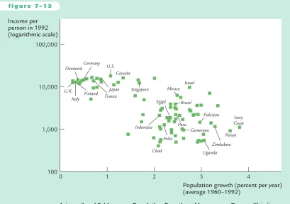
Wed, Feb 13, 2002 9:49 AM

Population growth (percent per year) (average 1960–1992)

International Evidence on Population Growth and Income per Person This fi

g-ure is a scatterplot of data from 84 countries. It shows that countries with high rates of population growth tend to have low levels of income per person, as the Solow model predicts.

Source:Robert Summers and Alan Heston, Supplement (Mark 5.6) to “The Penn World Table (Mark 5): An Expanded Set of International Comparisons 1950–1988,’’Quarterly Journal of Economics(May 1991): 327–368.

C A S E S T U D Y

Population Growth Around the World

Let’s return now to the question of why standards of living vary so much around the world. The analysis we have just completed suggests that population growth may be one of the answers. According to the Solow model, a nation with a high rate of population growth will have a low steady-state capital stock per worker and thus also a low level of income per worker. In other words, high population growth tends to impoverish a country because it is hard to maintain a high level of capital per worker when the number of workers is growing quickly. To see whether the evidence supports this conclusion, we again look at cross-country data.

(25)

26821

Wed, Feb 13, 2002 9:49 AM

7-4

Conclusion

This chapter has started the process of building the Solow growth model. The model as developed so far shows how saving and population growth determine the economy’s steady-state capital stock and its steady-state level of income per person. As we have seen, it sheds light on many features of actual growth experi-ences—why Germany and Japan grew so rapidly after being devastated by World War II, why countries that save and invest a high fraction of their output are richer than countries that save and invest a smaller fraction, and why countries with high rates of population growth are poorer than countries with low rates of population growth.

What the model cannot do, however, is explain the persistent growth in living standards we observe in most countries. In the model we now have, when the economy reaches its steady state, output per worker stops growing. To explain persistent growth, we need to introduce technological progress into the model. That is our first job in the next chapter.

Summary

1._{The Solow growth model shows that in the long run, an economy}_’_{s rate of}

saving determines the size of its capital stock and thus its level of production. The higher the rate of saving, the higher the stock of capital and the higher the level of output.

2._{In the Solow model, an increase in the rate of saving causes a period of rapid}

growth, but eventually that growth slows as the new steady state is reached. This conclusion is not lost on policymakers. Those trying to pull the world’s poorest nations out of poverty, such as the advisers sent to developing nations by the World Bank, often advocate reducing fertility by increasing education about birth-control methods and expanding women’s job opportunities. Toward the same end, China has followed the totalitarian policy of allowing only one child per couple. These policies to reduce population growth should, if the Solow model is right, raise income per person in the long run.

The Supply and Demand for Goods

*26797*

7

*26798*

7-1

The Accumulation of Capital

The Supply and Demand for Goods

*26799*

*26800*

*26801*

Growth in the Capital Stock and the Steady State

*26802*

d

d

d

d

D

d

D

D

d

D

*26803*

Approaching the Steady State: A Numerical Example

*26804*

d

d

D

D

d

*26805*

d

d

D

*26806*

How Saving Affects Growth

*26807*

*26808*

*26809*

7-2

The Golden Rule Level of Capital

Comparing Steady States

*26810*

d

d

d

d

*26811*

d

d

d

d

d

d

d

d

d

d

d

d

d

*26812*

Finding the Golden Rule Steady State:

A Numerical Example

d

d

*26813*

d

d

d

d

*26814*

d

The Transition to the Golden Rule Steady State

*26815*

*26816*

7-3

Population Growth

*26817*

The Steady State With Population Growth

26797

26798

26799

26800

26801

26802

_d

_d

_d

_D

26803

26804

_d

_d

_D

26805

_d

_D

26806

26807

26808

26809

26810

_d

_d

_d

26811

_d

_d

_d

_d

_d

_d

_d

_d

_d

_d

_d

_d

_d

26812

_d

26813

_d

26814

26815

26816

_{Population Growth}

26817

_d

_d

_d

_d

26818

_d

26819

_d

_d

_d

_d

26820

26821