Silvia Sari Busnitaa , Rina Oktaviani

(1)

International Journal of Agricultural Sciences. 1 (1):1-11 (2017)

* Corresponding email: silvia.busnita10@gmail.com

Research Article

How far climate change affects the Indonesian paddy production and

rice price volatility?

Silvia Sari Busnita

a*

_{, Rina Oktaviani}

b

_{, Tanti Novianti}

c

a_{Graduate school of Economics Department, Bogor Agricultural University, Bogor Indonesia, 16680.}

b_{Department and Director of International Trade Analysis and Policy Studies (ITAPS) Faculty of Economics and}

Management, Bogor Agricultural University, Bogor Indonesia, 16680.

c_{Department of Economics, Bogor Agricultural University, Bogor Indonesia, 16680.}

ARTICLE INFO

Article history:

Received 1 February 2016 Revised 28 May 2016 Accepted 20 July 2016 Keywords:

Climate change Paddy production Rice price volatility ARCH-GARCH VECM

A B S T R A C T

Food security issue after 2008 global-crisis is something relate with the climate change phenomenon which had worsened on the last few decades. The impact of global climate change can be seen from the fluctuation of main crops production yield in tropical countries. This has affected the food price fluctuations particularly on the grain price, both international and domestic markets. The rice-commodity, known for its thin market characteristics, is now also experiencing the fluctuation of production, its productivity and also the rice price. Considering the importance of rice as the main staple food in Indonesia, the purpose of this research is to identify the Indonesia’s rice price fluctuation (volatility) and to investigate how far climate change affects the Indonesian paddy production and rice price volatility. By applying monthly time-series data from 2007 to 2014, this research used ARCH-GARCH methods to find out the rice price volatility and VECM (Vector Error Correction Model) to investigate the impact of climate change phenomenon on the Indonesian paddy production, as well as rice price volatility both in the short-run and long-run. The result is important for the stakeholders and government in preventing the risk and uncertainty condition of paddy production and rice price fluctuation caused by climate change

1. INTRODUCTION

In recent years, there has food security issue growing along with the emergence

problems called 3F-crisis (food, fuel, and

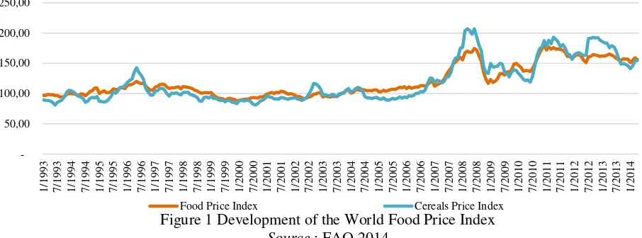
financial crisis) as the spillover effects of 2008 global crisis. This resulted in food prices surge at the consumer level around the world. Figure

1 shows the rise in world food price index,

which is largely dominated by the rising prices of cereals.Based on World Bank Trade Sector Development report (World Bank, 2011), from the sub-indices of international food prices, the price of grain first increased dramatically (in the last 30 years) during the early period of 2008 crisis.

Meanwhile, in the last decadesthere had

been increasingfloods and periods of drought, devastating cyclones, water, soil and land

resources that are continuing to decline in several parts of the World (IRRI, 2006). The

IPCC 4th Assessment Report (IPCC,

2007)statedthat Southeast Asia was expected to

be seriously affected by the adverse impacts of climate change. It is projected that by 2100 the annual mean temperature in Indonesia, the

Philippines, Thailand and Vietnam are going to

rise by 4.8 °C, with the global mean sea level

increasingby 70 cm during the same period (ADB, 2009). Since most of its economy relies on agriculture and natural resources as primary income, climate change has been and will continue to be a critical factor affecting productivity in the region above.

(2)

Figure 1 Development of the World Food Price Index

Food Price Index Cereals Price Index by 2030, while the rainfall patterns are

predicted to change, with the rainy season ending earlier and the length of the rainy season becoming shorter (FPRI 2011). Some empirical

studies have been done to analyze this phenomenon. Climate change affects all economic sectors, but the agricultural sector is generally the hardest hit in terms of the number

of poor affected (Rina Oktaviani, 2011). There

have been changes in precipitation and cycles of droughts and floods triggered by the Australasia monsoon and by the El Niño Southern Oscillation (ENSO) for the past three decades in Indonesia(Naylor R. L.,

2007; Boer, 2010). Thus, this has led to

agricultural production damage, causing

negative consequences for rural incomes, food prices, and food security in Indonesia.In Indonesia case,rice is one of the most important staple foods for more than half of the world’s population (IRRI, 2006)and influences the livelihoods and economies billions of

people in Asia. A recent study by the International Food Policy Research Institute

(IFPRI, 2012), titled ‘Climate change:Impact

on agriculture and costs of adaptation’,

highlighted some of the anticipated costs of climatechange, which one of them is the increasing prices in 2050 by 90% for wheat, 12% for rice and 35% for maizeon top of already higher prices.Indonesia's own position is the world's largest rice importer as 14% of the rice traded in the world (Indonesia’s Ministry of Trade,2012). Indonesia’s per capita

rice consumption is recorded still quite high,

reaching averagely 6.18 kg a week or 139.15 kg/capita/year (Central Statistical Bureau, 2014). This value is much higher than the ideal consumption by the developed countries standards as 80-90 kg/capita/year.Since the biggest consumption of Indonesian people is

gotten from rice, then it becomesmain concern

if the price became fluctuated.

.

Despite the large literatures that have examined

local food pricesin developing countries, there

is limited systematic evidence onthe

relationship between domestic weather

disturbances andlocal food prices (Baffes and Dennis 2013; Garg et al., 2013; Hazell 2013; Trostleet al., 2011; Von Braun, 2008; Webb, 1992).Climate change is likely to increase weather variability and incidences of extreme events (IPCC, 2012), potentially leading to growing impacts of weather shocks on agricultural and food price (Torero, 2010)). Especially in Indonesia, although the effects of-climate change already became such a reality in Indonesia, however to date there has few studies that have assessed the impacts of

current and forecast future climate change on the agricultural economic variables. Therefore, the primary objective of this paper is to calculate the fluctuation of Indonesian rice price (the volatility) especially after the 2008 crisis and to investigate the consequences of

global climate change on Indonesian paddy

(3)

SILVIA SARI BUSNITA,RINA OKTAVIANI, AND TANIA NOIANTI 3

Granger causality test to find out the relationship between the economics variables). Finally, the empirical results of this single country study may be helpful in guiding policy makers in devising long term sustainable agricultural economics policy in Indonesia.

This paper structure as follows:

Introduction section provides an overview of climate change impacts and food price surges after 2008 global crisis. Data and methods section describes the data and sources, and explain the econometrical approach to examine: (a) the Indonesian rice price volatility; (b) the impact of climate change on paddy production and its rice price fluctuation in Indonesia. Results and Discussion section presents and discusses the estimation result of:(a) Indonesian rice price volatility,(b) how far this climate data covering the time period from January 2007 to December 2014. This particular period was chosen because of the existence of 2008 global

price spikes over agricultural products

(domestically and internationally). Although there is still no evidence that weather shocks alone have played a major role in the food price spikes in 2008 (Headey, 2008), it seems, however, that they have contributed to the price spikes in interaction with other factors (Mitchell, 2008); von Braun & Tadesse, 2012). Therefore, the variables used in the study are following:

Table 1. List of Variables

Variable names Unit Symbol Source

Indonesia rice price volatility - Volatility Author Calculation using E-Views 8 Indonesia domestic rice price Rp / Kg LN HRG BRS Indonesia Central Statistical Bureau (BPS) Indonesia paddy production Quintal LNPRODUKSI Indonesia Central Statistical Bureau (BPS) Temperature (ENSO Index) ° C SUHU Climate Prediction Center (CPC)

Indonesian Rice Price (therefore

abbreviated as LN HRG BRS) – is the

Indonesian domestic rice price (consumer retail price) from main traditional markets from all over the provinces. While climatologists examine weather patterns and other data from the past in order to make predictions about earth's overall climate in the future (Akhmad 2014), here in this study we use the temperature data described by El Niño Southern Oscillation (ENSO) Index NINO 3.4,since it was the major factor influencing the year-to-year variation in rice production (Naylor R. L., 2001).

2.2 Methodological Frameworks

 ARCH-GARCH

The need for accurately assessing price volatility appears especially from the high level

of risk and uncertainty created for producers,

consumers and policymakers worldwide(Popa,

2013). Therefore, some reviews of the

econometric literature permitted the

identification of several methods implemented for estimating price volatility, from rather simple ones (like unconditional standard

deviation or the coefficient of variation) to more complex ones (such as the ARCH models). The modeling of volatility in time series has been revolutionized by the introduction of the Autoregressive Conditional Heteroskedasticity (ARCH) models by(Engle RF, 1987)and their generalized form (GARCH) by (Bollerslev,

1986)).The Generalized Autoregressive

Conditional Heteroscedasticity models

(GARCH) are applied in most of the literature studies (i.e.: food chains, energy-agricultural

commodity markets),which suggest that these

models are standard in price volatility modelling (ULYSSES WP 4). Numerous authors, as for example (Jordaan, 2007), Figiel and Hamulczuk (2010), Pop and Ban (2011), Apergis and Rezitis (2011), argue in favor of GARCH models on the grounds that they have the merit of accounting for both the predictable and unpredictable components in the price process, being also capable of capturing various dynamic structures of conditional variance and of allowing simultaneous estimation of several parameters under examination.

(4)

homoscedasticity assumptions (Firdaus, 2011.)Volatility based models ARCH (m) assumes that the data variance fluctuations are influenced by a number of “m” data fluctuations

before. As it has been told before, the ARCH

model is then generalized to GARCH by Bollerslev (1986). GARCH (r, m) assumes that

the data variance fluctuations are influenced by

a number of previous m data fluctuation and volatility of the previous amount of data r. The following is the general form GARCH (r, m) in this study:

𝒉𝒕=K+𝜹𝟏𝒉𝒕−𝟏+ 𝜹𝟐𝒉𝒕−𝟐+ ⋯ + 𝜹𝒓𝒉𝒕−𝒓+

𝜶𝟏𝜺𝒕−𝟏𝟐 + 𝜶𝟐𝜺𝒕−𝟐𝟐 + ⋯ + 𝜶𝒎𝜺𝒕−𝒎𝟐 (1)

In its general form above, a GARCH (r, m) model includes two equations, one for conditional mean and one for conditional

variance. The coefficients of ARCH-terms 𝜺_𝒕−𝒎𝟐

reveal the volatility of previous periods of time, measured with the aid of squared residuals from the equation of mean, and the coefficients of

GARCH-terms 𝒉_𝒕−𝒓show the persistence of

passed shocks on volatility. While 𝒉_𝒕 is variable

of log rice price at time t; K is constant variance; 𝜶𝟏, 𝜶𝟐… , 𝜶𝒎is coefficient of orde m that are

being estimated; 𝜹_𝟏, 𝜹_𝟐… , 𝜹_𝒓 is coefficient of

orde r that are being estimated. Having obtained

the best model of ARCH-GARCH, then the following model is used to estimate the value of

future volatility(𝛇_𝐭−𝟏) from an economic

 Vector Auto Regression (VAR/VECM)

VAR modeling is a form of modeling used for multivariate time series in which exogenous and endogenous are indistinguishable because of all endogenous variables (variables whose value are determined in the model). In accordance with Sims (1972), the variables used in the VAR equation were selected based on relevant economic theories and only endogenous variables were included in the analysis. This economics model is chosen because it meets four important things to be obtained from the establishment of economic modelling, namely: data description, forecasting, structural inference, and policy analysis. VAR /VECM

model created by Sims (1972) basically provides a tool for the four kinds of quantitative analysis: a) Forecasting, b) Granger Causality Test, c) Impulse Response Function (IRF),d) Forecast Error Decomposition of Variance (FEDV).

Compared to all other techniques that utilize time series data, it is essential to distinguish it unless the diagnostic tools used account for the dynamics of the link within a sequential ‘causal’ framework, the intricacy of the interrelationships involved may not be fully confined (Akhmad 2014). For this rationale, there is a condition for utilizing the advances in

time-series version. According previous

research(Akhmat, 2014), the following

sequential procedures are adopted as part of this methodology.

In order to confirm the degree, these series split univariate integration properties; we

execute unit-root stationarity tests. The

Augmented Dickey–Fuller(ADF)is suitable

testing procedure that is based on the null hypothesis that a unit root exists in the

autoregressive representation of the time series. This is because the time series data is often plagued with non-stationarity in levels, hence, the estimation based on such series usually provides spurious results(Azhar Khan M, 2014). Therefore, the first step in any time-series analysis is to examine the presence of unit roots in the underlying series, so that the problem of spurious relationships among variables can be removed. Dickey and Fuller (1979) devised a procedure to formally test non-stationarity which does not take into account high order auto correlation and hence limits the power of the

test. The Augmented Dickey–Fuller (ADF) test

is used to test the stationarity of the series. It is a standard unit root test which analyzes the order of integration of the data series. These tests have a null hypothesis of non-stationarity against an alternative of stationarity.

The next step is to choose the optimal lag

(5)

For investigating the long-run relationship

among variables, the Johansen co-integration test can be employed which is a two-step-procedure. In the first step, the individual series are tested for a common order of integration. If the series are integrated and are of the same order, they imply co-integration(Pesaran MH, 2001). In the second step, Johansen' co integration tests are applied on the series of same order of integration i.e.(1)series which determine the long run relationship between the variables. When the series that are co- integrated are of order 1, at race test (Johansen'sapproach) indicatesauniquecointegratingvectoroforder1and hence indicates the long run relationship. In the multivariate case, if the I (1)variables are linked by more than one co-integrating vector, the(Engle R F, 1987)procedure is not applicable. The Johansen and Juselius method has been developed in part by the literature available in the field and reduced rank regression. The

co-integrating vector ‘r’ is defined by Johansen as

the maximum Eigen-value and trace test. Johansen and Juselius (Johansen S, 1990)

proposed that the multivariate eco-integration methodology can be defined in the following general VAR model form:

Volatility

_t

=

𝒇

(

𝑺𝑼𝑯𝑼

t

,LOG_PRODUKSI

t

,

)

This study investigates the influence of climate change on paddy production and rice price volatility from two perspectives. One is to conduct the Johansen co integration tests to

explore the influencing directions among

climate changes, rice price volatility, and paddy production respectively. The other is to compare the influencing magnitude of climate change on paddy production and rice price volatility, based on the vector error correction model (VECM) and variance decomposition approach (FEVD. VECM itself is a form of VAR being restricted (restricted VAR).This additional restriction should be granted because of the existence of not stationary data but co-integrated. If the data is not stationary in levels but being stationary at its difference, then it must be examined whether the data used in the model has a long-term relationship or not. The existence or absence of a long-term relationship between the variables in the VAR system can be determined by performing integration test. If there is co-integration, the model used would be Vector Error Correction Model (VECM). VECM specification restricts the long-term relationship of endogenous variables that converge into its co-integration relationship, but still allows for

the existence of short-term dynamics. VECM

models used in this study are:

[

∆𝐿𝑜𝑔_𝑃𝑟𝑜𝑑𝑢𝑘𝑠𝑖

∆𝑉𝑜𝑙𝑎𝑡𝑖𝑙𝑖𝑡𝑦

∆𝑆𝑢ℎ𝑢

] = [

𝑎

10

𝑎

20

𝑎

30

] + [

𝑎

1121

… 𝑎

1323

𝑎

31

… 𝑎

33

] + [

∆𝐿𝑜𝑔_𝑃𝑟𝑜𝑑𝑢𝑘𝑠𝑖

∆𝑉𝑜𝑙𝑎𝑡𝑖𝑙𝑖𝑡𝑦

𝑡−1𝑡−1

∆𝑆𝑢ℎ𝑢

𝑡−1

] + [

𝑒

1𝑡2𝑡

𝑒

3𝑡

]

(4)

with 𝑎₁₀-𝑎₉₀ as the constanta; 𝑒_1𝑡-𝑒_3𝑡 as the error term; and 𝑎₁₁-𝑎₃₃ (𝑎_𝑖𝑗) as the lag coefficient of

j-variables for the-i equation.

3. RESULTS AND DISCUSSION

In this section, we analyze the evolution of consumer retail price for Indonesian domestic rice market sourced from Indonesian Central Bureau of Statistics (BPS). As an overview of-

(6)

0

Indonesia Consumer Retail Price of Rice (Rp/Kg)

45,00

2004 2005 2006 2007 2008 2009 2010 2011 2012 2013 2014 2015

It can be seen the prices continue to move up slowly starting at the end of 2009 and keeps

fluctuating in the increasing trends. This is something different from the international rice price condition as reported by the World Bank

(2011) that there was high spike in world rice prices on April and May 2008 which the world rice price reached even three times higher than different condition of Indonesian domestic rice prices and world rice prices mainly resulted

Figure. 2 Indonesia Consumer Retail Priceof Rice January 2007 – May 2015

Source: Indonesia Central Statistic Bureau 2015

It can be seen the prices continue to move up slowly starting at the end of 2009 and keeps

fluctuating in the increasing trends. This is something different from the international rice price condition as reported by the World Bank (2011) that there was high spike in world rice prices on April and May 2008 which the world rice price reached even three times higher than different condition of Indonesian domestic rice prices and world rice prices mainly resulted

Figure 3 Indonesia PaddyYield 2005 – 2014 (Qu/Ha)

Source: MinistryofAgriculture 2015

(7)

* Corresponding email: silvia.busnita10@gmail.com 0,000000

0,001000 0,002000 0,003000 0,004000

2007… 2007… 2007… 2007… 2008… 2008… 2008… 2008… 2009… 2009… 2009… 2009… 2010… 2010… 2010… 2010… 2011… 2011… 2011… 2011… 2012… 2012… 2012… 2012… 2013… 2013… 2013… 2013… 2014… 2014… 2014… 2014…

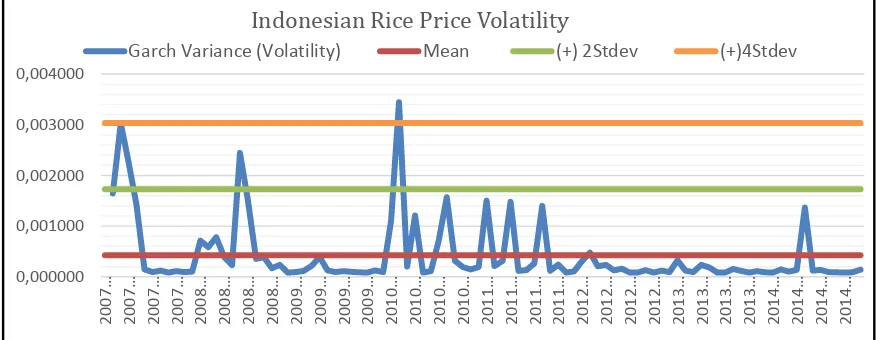
Indonesian Rice Price Volatility

Garch Variance (Volatility) Mean (+) 2Stdev (+)4Stdev

In the specification of ARCH-GARCH models to measure the rice price volatility, there are 2 main stages that must be done: 1)

Identification and model determination (mean

equation); 2) Identification and determination of ARCH-GARCH models. Stage (1) includes testing data stationery, determining a tentative ARIMA models to estimate the parameters and the selection of the best model. The following table test shows the best ARIMA model and ARCH-GARCH best selected models.

Based on Table 2, it can be seen that the

Indonesian rice prices have the ARCH effect. This is shown in prob. F value which is greater than the critical value 0.05, while the applications of ARCH-GARCH models can only be done for the variable of world rice price and Indonesia’s rice price to further know its volatility. This measure of volatility is then shown by the conditional standard deviation which is root of variance of the ARCH-GARCH best selected models which had been estimated.

Table 2. ARCH-GARCH Model Specification Result

*_{) Level of significance at 5%}

Source: Authors’ calculations in EView

3.2 The Volatility of Indonesia Domestic Rice Price

In this study, monthly data between January

2007 and December 2014 have been used to

analyze as accurately the recent developments as possible. A series of steps required by the statistical analysis of the time series were

initially implemented. Based on author’s estimation result using Eviews 8, Indonesian rice price volatility values over time showed the variation among diverse enough (time varying) from 2007 to 2014.

Figure 4 Indonesian Rice PriceVolatility Source: Authors’ calculationusingEviews 8.

The fluctuations in the prices of rice during

the period January-April 2007 and 2008, allegedly in addition to the effects of the world food crisis as well as the phenomenon of

increased demand public holiday such as Christmas and New Year. Government intervention to stabilize the price of rice through a market operation seems to be successful in the Testing Non-Stationary Determination ARIMA

model Determination ARCH-GARCH Model t-Statistic Prob* Best ARIMA Prob.F * ARCH Effects

(?)

Best ARCH model

LOG HRG BRS -2.01138 0.5873 - - - -

D (LOG HRG

BRS) -8.71190 0.0000

ARIMA

(0,1,1) 0.0000 Yes ARCH (1,0)

(8)

short term. But in early 2010 until the end of 2011 and then (Figure 4) return fluctuation is sharply enough to reach twice the value of the standard deviation. The price of rice beginning to stabilize at the end of the year 2008 was on account of production and reserves adequacy domestic rice stocks to meet the needs of society

at that time.

However, the termination of restrictions on rice exports beginning in late 2009— accompanied by the opening of the flow of imported rice into the country—made domestic rice prices fluctuated throughout 2010 and 2011 and then. On the other hand, the national rice production in 2010 and 2011 did not experience a significant increase compared to the need for consumption of rice showing steady increase each year.

While the Indonesian rice prices reached the

highest level of disparity in 2007, it indicates some spikes per monthly period during the year

2007.Domestic rice price disparity levels high enough can also be seen in 2010 and 2011, which reached a value above 50%.This means that there is a change in the rice price increase until it reaches 50% of the average change in the price of ordinary rice. On the one hand, the level of inequality in rice prices is also due to the inclusion of rice imports into the domestic market. Due to high level of gap between

domestic rice prices that have been mixed with

the price of imported rice, a new domestic

equilibrium price that would be different when compared to the previous period will be formed.

3.3 Pra-estimation Test Result of VAR/VECM

Pra-estimation testing is held before estimating VAR / VECM. The present study

performs the Augmented Dickey–Fuller (ADF)

unit root tests for variables with regard to their stationary properties.

The results of the unit root test on the level of ADF test showed that LOG PRODUKSI variables are not stationary in levels. Thus, unit

root test is then performed on the first difference

from the results of all the variables stationary on the level of 5%. Based on the optimum lag testing, testing criteria based on SC (Schwartz Criterion) minimum value showed optimum models in lag 4. Testing of stability VAR also showed all the roots polynomial function unit have a value of less than 1. This means that the VAR model is so stable that the Impulse Response Function Analysis (IRF) and Forecast Error Decomposition (FEVD) are considered valid. The next stage is testing the co-integration using Johansen Co-integration test (1988) with the following results.

.

Table 3 The unit root test results

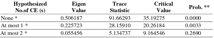
Table 4 Johansen Co-integration test results

*denotes rejection of the hypothesis at the 0.05 level **MacKinnon-Haug-Michelis (1999) p-values

Based on the result of trace test in Table 4, it indicates 2 co-integrating equations at the 0.05 level. This also means that climate change

(specifically temperature variable) hasat least

one co integration relationship with paddy

production and rice price volatility at5% level.

3.4 Analysis Response of Indonesia’s Rice Price Volatility and Paddy Production towards Climate Change

This analysis is used to see the response of

Hypothesized No.of CE (s)

Eigen Value

Trace Statistic

Critical

Value Prob. **

None * 0.506187 91.66293 35.19275 0.0000

At most 1 * 0.225723 28.15910 20.26184 0.0033

(9)

International Journal of Agricultural Sciences. 1 (1):1-11 (2017) an endogenous variable to shock, whether

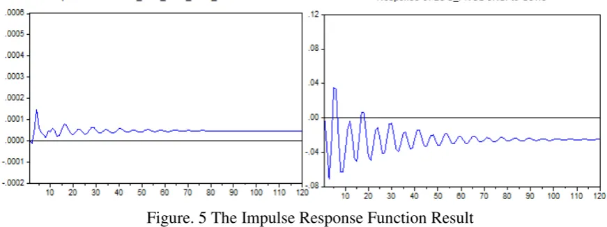
transmitted by the variable itself or by other variables in current time and in the future. In analysing the response of Indonesian rice price volatility and paddy production towards temperature changes, we projected the time period as of 120 months (10 years) ahead. This is because in previous studies, the climate change effect seems to have long-run impact on the variables on the study. Following picture (Figure 5) is the Impulse Response Function results describing the shocks of temperature variable towards the Indonesia’s paddy production and its rice price volatility.

Following are the detailed explanation:

Shocks on the Indonesia’s temperature changes

would be responded negatively by the paddy production variables. Even though it will have positive respond in the early-12 month but in the long term such temperature changes would have negative impact on the paddy production. This is similar to the previous study (Naylor R. L., 2001) as the temperature changes plays a major factor in influencing year-to-year variation in rice production. The response of this temperature change is likely to be reduced and stable on the 116 months in the level -0.026 percent.

Shocks on the Indonesia’s temperature

changes would be generally responded

positively by the rice price fluctuation (volatility). The greater the changes of the temperature, the higher fluctuation would be. The rice price fluctuation would reach its stable stages starting the period of 60 months as the average level would be at 0.00004 and/or 0.00005 percent.

The FEVD simulation results (Table 5) show that overall in the short term the most dominant variant contributing in explaining the Indonesian paddy production is the paddy production shock itself (approximately 52percent in the early 12months period), followed by the temperature changes (reaching 38.39 percent on the same period above).The contribution of the temperature to the paddy production variable is theoretically explained from the supply side. Mean while the most dominant variant contribution in explaining the Rice price volatility is also the rice price volatility itself, (approximately 72 percent in the early 12 months period), then followed by the paddy production variables (reaching 21.01 percent). The temperature changes only contribute approximately 6.17 percent to it. This means that the direct factor that influences the rice price fluctuation is still the paddy production, as it was derived from the supply side factors affecting the rice price in Indonesia.

Figure. 5 The Impulse Response Function Result

Source:

Authors’

calculation using EViews 8

Table 5. The Variance Decomposition Result

Variable(s) _{(%) between Temperature Changes}Variance decomposition analysis _{influence to changes of its variable}Highest contributing factor

LOG_PRODUKSI 38.29 % LOG_PRODUKSI (52.82%)

(10)

Based on this FEVD result, it can be said that in the short run, the greatest response of all the particular variable is actually derived from the variable shocks itself. This is consistent with the random walk theory of the rice price

movements that have distribution and

interdependence with one another. This condition

would be vice-versa as the periods added in the

long run.

4. Conclusion and Policy Implications

This study measures the volatility of

Indonesia domestic rice price and examines how far the climate change (temperature change) affects Indonesian paddy production and its rice price volatility for the 2007-2014 periods of time. The results find that the volatility (fluctuation) in Indonesian rice price variable and time varying, with the highest price spikes happened on 2010 and 2011 respectively existed. While the next result showed that the climate changes (the temperature changes) would affect negatively the paddy production in Indonesia both in the short

run and long run. However, the temperature changes would positively influence the rice price fluctuation in Indonesia. All of the results match exactly compared with the previous similar research and related theories. Therefore, the policy implication of this result is, it is important to the government to prioritize the efficiency of rice price stabilization policy as one of the controlling prices mechanisms, especially when there was natural disaster because of the climate change (i.e.: drought, floods, etc.). Also, a public stockholding act is urgent to be realized soon considering their important role in maintaining the domestic food stock reserves. In addition, for long-term productivity improvement programs should be optimized properly, such as: the irrigation system reparation and management, agricultural subsidies improvement, farmers training on the field for using technology, and a better management of production, so that the productivity of paddy and rice is evenly

distributed throughout the whole harvest area in Indonesia.

REFERENCES

ADB. (2009). The Economics of Climate Change

in Southeast Asia: A Regional Review. Manila: ADB (Asian Development Bank).

Akhmat, G. (2014). Does energy consumption

contribute to climate change? Renewable

and Sustainable Energy Reviews 36,

123–134.

Azhar Khan M, Z. K. (2014). Global estimates of energy consumption and greenhouse gas

emissions. Renewable Sustain Energy

Review.

Boer, R. (2010). Climate Change and

Agricultural Development: Case Study in Indonesia. Unpublished Report.: Paper commissioned by International Food Policy Research Institute.

Bollerslev, T. (1986). Generalised Autoregressive

Conditional Heteroskedasticity. . Journal

of Econometrics, 31 (3). pp. 307-327. Amsterdam: North Holland and Elsevier Science Publishers BV.

Dickey D, F. W. (1979). Likelihood ratio statistics for autoregressive time series

with a unit root. Journal of the American

Statistical Association, (2):427–31. Engle R F, G. C. (1987). Co-integration and

error-correction:representation,estimation

and testing. Econometrica 55(2), 251–76.

Engle RF, G. C. ( 1987). Co-integration and

error-correction: representation,

estimation and testing. Econometrica., 55

(2) : 251–76.

Firdaus, M. (2011.). Applications To

Econometrics Panel Data and Time Series. Bogor (ID): IPB Press.

IPCC. (2007). Contribution of Working Group III

to the Fourth Assessment Report. Cambridge, UK: Cambridge University Press.

IRRI. (2006). Bringing hope, improving lives:

Strategic Plan 2007–2015. Manila: IRRI. Johansen S, J. K. (1990). Maximum likelihood

estimation and inference on

cointegration: with application to the

demand for money. Oxford Bulletin Econ

Stat, 169-210.

Jordaan, H. G. (2007). Measuring the price volatility of certain field crops in South

Africa using the ARCH/GARCH

approach. Agrekon, 46(3), p. 306-322.

Naylor, R. L. (2001). Using El Niño/Southern Oscillation Climate Data to Predict Rice

Production in Indonesia. Climatic

Change 50: 255–265.

Naylor, R. L. (2007). Assessing Risk of Climate Variability and Climate Change for

Indonesian Rice Agriculture.

(11)

Sciences of the United States of America (PNAS) 104 (19), 7752–7757.

Pesaran MH, S. Y. (2001). Bounds testing approaches to the analysis of level

relationships. Journal of Applied

Econometrics, 16(3):289–326.

Popa, L. N. (2013). The Challenges of Sugar Market: An assessment from the Price

Volatility Perspective and Its

Implications for Romania. Procedia

Economics and Finance 5, 605-614 doi: 10.1016 / S2212-5671 (13) 00071-3. Rina Oktaviani, S. A. (2011). The Impact of

Global Climate Change on the

Indonesian Economy. IFPRI Discussion

Paper 01148.

World Bank. (2011). Developments, Drivers and

Impact of Commodity Prices: Implications for Indonesia's Economy.

Jakarta: World Bank.